| |
SYSC 4405 - Digital Signal Processing
Midterm #2: Material is 2−12,14−25
Midterm #1 (with solutions):
V1
V2
Midterm #2 (with solutions):
[pdf]
Marks (by last 3 digits of student number)
Discrete time signal and system representation: time domain, z-transform,
frequency domain. Sampling theorem. Digital filters: design, response,
implementation, computer-aided design. Spectral analysis: the discrete
Fourier transform and the FFT. Applications of digital signal processing.
Prerequisites
SYSC 2500 or SYSC 3500 or SYSC 3600.
Students who have not satisfied the perquisites for this course must either
a) withdraw from the course, or b) fill out a prerequisite waiver from
www.sce.carleton.ca/ughelp, or
c) may be deregistered from the course after
the last day to register for courses in the term.
Instructor
|
Andy Adler
| |
Email: adler@sce.carleton.ca
|
|
Note: Emails to the instructor must contain
a subject line "SYSC4405: your subject line"
| |
Office: Canal 6204
| |
Phone: +1-613-520-2600 x 8785
| |
Office Hours: Thursday 1315−1445
|
|
|
Teaching Assistants
| T.A.:
| Patrick Quesnel,
|
| Kun Wang
| | Email:
| patrickquesnel@cmail.carleton.ca
|
| KunWang@cmail.carleton.ca
|
|
Office
|
Canal 6107
|
|
ME 4324
|
|
Office Hours:
|
Thurs 11:30−12:30
|
|
Tues 10:00−11:00
|
Times and Locations
Fall 2012
(Sept. 10 − Dec. 3)
| Section |
| Activity |
| Day |
| Time |
| Location |
|
|
SYSC4405
| |
LEC
| |
Mon
| |
13:05−14:25
| |
TB 238
|
|
|
| |
LEC
| |
Wed
| |
13:05−14:25
| |
TB 238
|
|
|
| |
LAB 1
| |
Mon (even weeks, starting Sept.17)
| |
14:35−17:25
| |
Canal 5107
|
|
|
| |
LAB 1
| |
Tues (Odd weeks, starting Sept.11)
| |
14:35−17:25
| |
Canal 5107
|
|
|
| |
LAB 1
| |
Thur (Odd weeks, starting Sept.13)
| |
14:35−17:25
| |
Canal 5107
|
|
Text
The text for this course will be the course slides. Links to
course slides are given on the corresponding schedule.
Recommended suplementary material.
Monson H. Hayes, Digital Signal Processing,
Schaum's Outlines, McGrawa-Hill
Steven W. Smith,
The Scientist and Engineer's Guide to Digital Signal Processing
California Technical Publishing
Additional Reference:
Course Notes (2006), Richard Dansereau
Marks
| Work |
| Value
|
|
Quizzes (in Lab)
| |
15%
|
|
Laboratories
| |
15%
|
|
Midterm Exams (#1 & #2)
| |
15%
|
|
Final Exam
| |
40%
|
Marks Policies
- Weighting of midterm and final will be optimized
within the range given to maximize student benefit.
- Late work Policy (without *excellent* excuse):
1) 20% if ≤ 7 days late,
2) 0 mark if > 7 days late.
- If you have a question about a mark you have received,
fill out, sign and submit
this form.
Students with Disabilities
The Paul Menton Centre for Students with Disabilities (PMC) provides services
to students with Learning Disabilities (LD), psychiatric/mental health
disabilities, Attention Deficit Hyperactivity Disorder (ADHD), Autism Spectrum
Disorders (ASD), chronic medical conditions, and impairments in mobility,
hearing, and vision. If you have a disability requiring academic accommodations
in this course, please contact PMC at 613-520-6608 or pmc@carleton.ca for a
formal evaluation. If you are already registered with the PMC, contact your PMC
coordinator to send me your Letter of Accommodation at the beginning of the
term, and no later than two weeks before the first in-class scheduled test or
exam requiring accommodation. After requesting accommodation
from PMC, meet with me to ensure accommodation arrangements are made. Please
consult the PMC website for the deadline to request accommodations for the
formally-scheduled exam.
Exams (Midterm and Final)
- Midterm exams are Oct. 22 and Nov. 19.
- Final exam date will be set by the university
- For all exams, you will be permitted a calculator and
one (1) 8.5"×11"
paper sheet containing any information you choose (double sided).
-
Previous Exams (for practice)
Final exam 2011,
Midterm exam 2011,
Final exam 2008,
Midterm exam 2008,
Midterm exam 2007 (with solutions − remove t in solution for Q#1),
Final exam 2007,
Practice exam 2007 (with solutions),
- Quiz solutions (2011):
Quiz#2 (error in Q#A, table for memoryless and causal),
Quiz#3,
Quiz#4,
Quiz#5A,
Quiz#5B,
Quiz Nov 14
Quiz Nov 28
Quizzes
Quizzes take place in the first 15 minutes of each
lab session. Each quiz will be one question from the
corresponding list below:
| |
| No. |
| Assignment |
| Due Date
|
|
1
| |
No quiz for this lab
| |
Sep. 11 (LAB1O)
Sep. 13 (LAB2O)
Sep. 17 (LAB1E)
|
|
|
|
2
| |
- Characterize whether following systems are:
a) Linear,
b) Shift Invariant,
c) Memoryless,
d) LSI,
e) Causal,
f) Stable:
- y[n]= 8x[n] + 2
- y[n]= x[n]
+ x[n−2]
+ x[n−4]
+ x[n−6]
+ x[n−8]
+ …
- y[n]= x[n] + x[0]
- y[n]= 0
- y[n]= 2x[n²]
- y[n]= (x[n²])²
- Given the sequence, x[n]
x[n] = 2δ[n+3] +
(3−n)(u[n]−u[n−3])
sketch the following sequences (for −2≤n≤8):
- y1[n] =
x[2n−3]
- y2[n] =
x[|n|]
- An LSI system responds to a step input (u[n])
with output (g[n]).
Calculate the unit sample (impulse)
response as a function of g[n].
- Can a LSI system be characterized completely by its
reponse to one test input signal? However, in practice,
it is not a good idea to only use one test to characterize a
system. Briefly (<50 words) describe why not
- A system is described by the LCCDE
y[n] − y[n−1]
+ y[n−2] =
x[n−3]
The input is x[n] =
n(u[n]−u[n−4]);
initial conditions are
y[−3] = 2 and
y[−4] = 1.
Show the response of the system from
n=−2 to n=+8.
- Q2 from Final 2011,
- Q3 from Final 2011,
- Q5 from Final 2011,
| |
Sep. 25 (LAB1O)
Sep. 27 (LAB2O)
Oct. 1 (LAB1E)
|
|
|
|
3
| |
Background: You're building a portable music recorder and playback system. The system has recorded a sample sound for playback.
The input, x(t), at the microphone is:
x(t)=
10 sin(600πt) +
5 sin(4100πt) mV
- Show the Fourier transform, X(Ω), as a phasor plot.
- Without using any type of anti-aliasing filter, the
signal is sampled at 1000 samples/s, giving a
sampled sequence x[n].
Calculate x[n] showing each
term in its lowest frequency form.
- Calculate the Nyquist frequency for this sampling rate,
and calculate at what frequency the aliased representation of
sin(4100πt) will appear in the sampled signal.
Is this signal aliased?
- Calculate the value of x[n]
for n = 0 … 3 .
- Input x[n] is sent into two filters:
Filter 1: y = f1(x):
y1[n] = ½(
x[n] +
x[n−1] )
Filter 2: y = f2(y):
y2[n] = ½(
x[n] +
y[n−1] )
Show the block diagram for each filter.
Calculate
y1[n] and
y2[n]
for n = 0 … 3,
and x[n] = δ[n].
Assume initial conditions are zero.
-
Calculate the impulse response
h1[n] and
h2[n], for each filter
- Given two filters:
f1:
y[n] = 2x[n−1] + 3x[n−3]
f2:
y[n] = x[n−1] + 0.4y[n−1]
f2
The filters are combined in
various ways. Calculate the impulse response of each filter,
h1[n]
and
h2[n].
-
Calculate the impulse response of
the following combined filters, in terms of x[n]
          ______   ______
i)  x --->| f1 |-->| f2 | ---> y
          ______   ______
ii) x --->| f2 |-->| f1 | ---> y
          ______   __
iii)x -+->| f2 |-->|+| ---> y
       |->| f1 |----^
| |
Oct. 9 (LAB1O)
Oct. 11 (LAB2O)
Oct. 15 (LAB1E)
|
|
|
|
4
| |
Consider the signal, x(t),
x(t)=
5 cos(2π200t) +
4 cos(2π300t) +
3 cos(2π400t) +
2 cos(2π500t) mV
- Show the Fourier Transform phasor plot of
x(t)
- Initially we sample x(t) at 700Hz.
Calculate x[n].
Is the signal aliased?
- Show the Fourier Transform phasor plot
of x[n]. Label each
aliased component as "Folded" or "Non-folding".
- If we consider the aliased components to be noise,
What is the signal to noise ratio?
(recall that the power of each phasor component is ½×Amplitude²)
- Calculate the DTFT, X(ω), of:
x[n]= u[n](0.1)n
- Calculate the DTFT, X(ω), of:
x[n]= u[n](0.1)n cos( 0.1n )
- Q5 from Practice Midterm (F08),
- Q6 from Practice Midterm (F08),
- Q8 from Practice Midterm (F08),
| |
Oct. 23 (LAB1O)
Oct. 25 (LAB2O)
Oct. 29 (LAB1E)
|
|
|
|
5a
| |
Note: These quiz questions are designed
to provide an example to practice for midterm #2.
This is too long for an 80 minute midterm, but the
questions will be similar.
Questions marks "(not for quiz)" are for midterm practice,
but not for the quiz 5A.
- A signal x(t) is zero everywhere
except for the range 1.0s<t<1.001s,
where it increases linearly from 0V to 1V.
A DSP system samples the signal at
FS=2.5kSamples/sec.
Sketch the signal, x(t) and x[n]
in range 1.0s<t<1.001s and indicate
the values of n and x[n]
- Consider system S
y[n] =
0.2x[n−2] +
0.3x[n−3] +
0.9y[n−1]
Sketch a block diagram of this system (in the
canonical form we saw in class)
-
Consider the input
x[n] = {1,2,3,4,0,0,0,0}
and initial conditions
y[−1] = 1.
Calculate
y[n] for 0≤n≤4
(to two signifcant figures).
-
Calculate
h[n] for System S
-
Calculate
H(ω) for System S
- We wish to calculate the convolution
( y[n]= h[n] * x[n] )
where
x[n]= {2,4,6,8,10,12,14,18}
h[n]= {2,−1}
- Using linear convolution, calculate
y[0] and
y[5]
- Sketch the convolution operation of the overlap-add method
using N=4, M=2, and B=3.
- Calculate
y[0]
using circular convolution, using the overlap-add approach.
- Calculate
y[5]
using overlap-add with and using circular convolution.
- (not for quiz) Implement circular convolution
using the DFT and IDFT of length N=4.
Use this value to Calculate
y[5]
- Given a DSP system with Ts=1ms,
we need a band pass FIR filter,
hBP[n],
which will
1) Accept frequencies in the range 80−120Hz (to within 10%)
2) Reject frequencies below 50Hz (by at least 50 dB)
3) Reject frequencies above 150Hz (by at least 40 dB)
- Calculate the center frequency and sketch
the filter requirements
- Calculate the ideal filter hideal[n].
- Choose a window w[n] to meet the requirements (use Slide 22.14).
- What is the FIR filter hBP[n]?
What is the delay (in ms) of this filter?
- To implement this filter as an FIR convolution,
how many multiplies and additions are required
per output sample.
- (not for quiz) Assuming additions take 1 clock cycle, and multiplies
take 10, what is the slowest clock speed DSP that
can be used for this application using convolution?
- (not for quiz) To implement this filter using FFT block processing,
calculate
how many multiplies and additions are required
per output sample for N= 2048.
- (not for quiz) What is the slowest clock speed DSP that
can be used for this application using the FFT and DSP block processing,
using N=2048?
|
Nov. 6 (LAB1O)
Nov. 8 (LAB2O)
Nov. 12 (LAB1E)
|
| |
|
|
5b
| |
We wish to implement a band-pass filter
to demodulate an AM radio station with
frequency content in the range
726−734kHz (content in this range
should be accepted ±1%). We need to reject
frequencies below 720kHz and above 740kHz
by at least 40dB. We use a A/D system
with a sampling frequency of 2MSamples/sec.
Our DSP takes 1 clk cycle for addition and
5 clk cycles for (complex) multiplication (assume other
operations are zero cost).
- Sketch the filter specifications. What
are ωp,L, ωp,H and
ωs,L, ωs,H?
- Calculate ωc,
ω0 for the BPF.
Calculate the ideal BPF.
- Choose a windowing function and window length
for this filter.
- Calculate the expression for the FIR filter
to implement this specification.
- To implement this filter as an FIR convolution,
how many multiplies and additions are required
per output sample.
- What is the slowest clock speed DSP that
can be used for this application using FIR convolution?
- To implement this filter using FFT block processing,
calculate
how many multiplies and additions are required
per output sample,
for N= 4096
- What is the processing delay for the FIR?
Consider a filter described by H(z) =
Y(z)/X(z), where
H(z) =
2z−2/(1 −
z−1 −
2z−2)
-
Given samples of x[n] = {1,2,3,4},
calculate the output y[n] for the filter
Assume zero initial conditions.
-
Factorize H(z) into a form
H(z) = Az−2/(1 −
az−1)
+ Bz−2/(1 −
bz−1)
-
Calculate the inverse z-transform h[n].
| |
Nov. 20 (LAB1O)
Nov. 22 (LAB2O)
Nov. 26 (LAB1E)
|
|
Laboratories
Lab attendance is a compulsory component of this course. Laboratories will
be three hours alternate weeks as per the registration schedule.
Attendance is compulsory.
Labs will consist of programming in MATLABtm,
developing filter models
in SIMULINKtm, and using the TI TMS320C6713 DSP starter kit board.
Students must do labs in groups of two. Lab results must
be shown to T.A. before the end of the lab period.
Course Outline
|
Date
|
|
Activity
|
|
|
Sep. 10,
Sep. 12
| |
Introduction to DSP:
Slides #0,
Slides #1,
Matlab Programming for DSP:
Slides #5,
Quantization:
Slides #13,
The Loudness War [Youtube],
|
|
Sep. 17,
Sep. 19
| |
Signals and Systems
−
Slides #2,
Slides #3,
Slides #4
Sound&Wave[Youtube],
Sonata Pathétique[Youtube]
Sep. 19: Guest Lecture:
Mako Hirotani:
Notes,
PRAAT Software
|
|
Sep. 24,
Sep. 26
| |
Fourier Analysis
− Slides #6,
Slides #7,
Slides #8,
Slides #9,
Slides #23,
DSP Examples:
Example #1,
Spectrogram View[Youtube],
|
|
Oct. 1,
Oct. 3
| |
Sampling
− Slides #10,
Slides #11,
Slides #12,
Antialiasing fonts:
Sub-pixel rendering,
Anti-aliasing
DSP Examples:
|
|
Oct. 8
| |
Class cancelled (Thanksgiving day)
|
|
Oct. 10,
Oct. 15
| |
Discrete Fourier Transform,
− Slides #14,
Slides #15,
Slides #16,
Slides #17,
|
|
Oct. 17
| |
Review:
Midterm Review (2011)
Practice Midterm (F08),
Midterm (+ solutions),
Midterm exam 2008,
Midterm exam 2007 (with solutions − remove t in solution for Q#1),
|
|
Oct. 22
| |
Midterm exam #1
|
|
Oct. 24,
Oct. 29,
Oct. 31
| |
FIR Filter Design
− Slides #18,
Slides #19,
Slides #20,
Slides #21,
Slides #22,
|
|
Nov. 5,
Nov. 7,
Nov. 12
| |
Spectrogram,
Fast Fourier Transform
− Slides #23,
Slides #24,
Slides #25,
|
|
Nov. 14
| |
Review
|
|
Nov. 19
| |
Midterm exam #2: Material is 2−12,14−25
Location: SA306
|
|
Nov. 12,
Nov. 21,
Nov. 26,
Nov. 28
| |
Z-Transform,
Transform analysis of systems,
Advanced topics
− Slides #28,
Slides #29,
Slides #30,
Slides #31,
Slides #32,
Slides #33,
|
|
Dec. 3
| |
Review,
|
|
Dec. 12
| |
Final Exam, 9:00−11:30 (AT 301)
|
Code Examples
Code examples given in class are listed here:
|
Date
|
|
Code
|
|
|
Sep. 12
| |
time = 0:300;
signal1 = zeros(1,100);
signal2 = linspace(4000,800,101);
signal = [signal1, signal2, signal1];
plot(time,signal,'k');

hold on; ylim([-1000,5000]);

sample_time = (0:6)*50 + 1;

thresh = -3500+1000*(0:6);
for i=1:length(sample_time)
  stime_i = sample_time(i);
  samp_i  = signal(stime_i);
  stem(stime_i, samp_i,'b');

  gt_thresh = samp_i > thresh;
  adcvalue    = sum( gt_thresh);
  repvalue    = (adcvalue-4)*1000;

  stem(stime_i,repvalue,'r')
  fprintf('%4d ',[i,samp_i, adcvalue,repvalue]);fprintf('\n');

end
hold off
|
|
Sep. 25
| |
Music from Brad Sucks.
Full song is available under Creative Commons license as
Making Me Nervous.
(Aside, the artist has a new record release,
if you're interested:
Brad Sucks Record Release @ Zaphods
November 2, 2012 - Ottawa, ON )
Step #1: Download sample: Sample (10.5s−18.5s)
[y,fs] = wavread('Brad_Sucks_-_Making_Me_Nervous_10s-18s.wav');
time = (0:length(y)-1)/fs;
ch1 = y(:,1)/2; ch2 = y(:,2)/2;

for r = [2,1,0.5];
  out1= ch1 * r; subplot(211); plot(time,out1); ylim([-1,1]);
  out2= ch2 / r; subplot(212); plot(time,out2); ylim([-1,1]);
  pause
  wavwrite([out1,out2],fs, ['Amplitude-',num2str(r),'.wav']);
end

Output:
Amplitude-0.5.wav,
Amplitude-1.wav,
Amplitude-2.wav

[y,fs] = wavread('Brad_Sucks_-_Making_Me_Nervous_10s-18s.wav');
for D = [50,100,300,1000,1e4];
  delay = zeros(D,1);
  out1 = [ch1; delay];
  out2 = [delay; ch2];
  wavwrite([out1,out2],fs, ['Delay-',num2str(D),'.wav']);
  out1 = [delay; ch1];
  out2 = [ch2; delay];
  wavwrite([out1,out2],fs, ['Delay+',num2str(D),'.wav']);
end


Output:
Delay+50.wav,
Delay+100.wav,
Delay+300.wav,
Delay+1000.wav,
Delay+10000.wav,
Delay-0.5.wav,
Delay-0.wav,
Delay-50.wav,
Delay-100.wav,
Delay-300.wav,
Delay-1000.wav,
Delay-10000.wav,
|
|
Oct. 1
| |
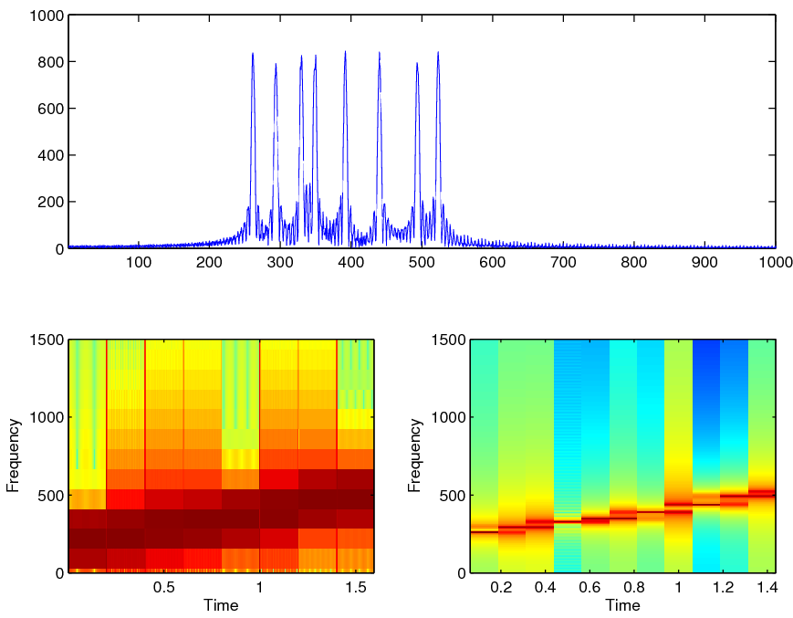
Samples from
Slides #23,
fs=8192; t=0:1/fs:0.2; x1=[];
notes=[3 5 7 8 10 12 14 15];
for i=notes;
x1=[x1 cos(2*pi*(220*2^(i/12))*t)];
end;
X1=fft([zeros(1,1000) x1 zeros(1,1000)]);
W=linspace(0, fs, length(X1));
subplot(211); plot(W,abs(X1)); xlim([1,1000]);
subplot(223); specgram(x1,64,fs); ylim([0,1500]);
subplot(224); specgram(x1,2048,fs); ylim([0,1500]);
print slides23-sound1.png
wavwrite(x1*.99,fs,16,'slides23-sound1.wav')
Output:
slides23-sound1.png,
slides23-sound1.wav
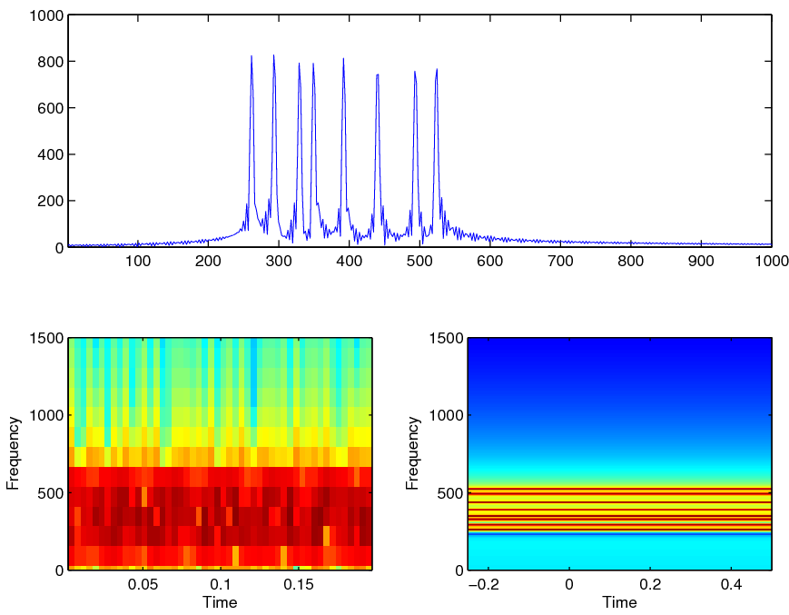
x2=zeros(1,length(t));
for i=notes;
x2=x2+cos(2*pi*(220*2^(i/12))*t);
end;
X2=fft([zeros(1,1000) x2 zeros(1,1000)]);
W=linspace(0, fs, length(X2));
specgram(x2,64,fs)
subplot(211); plot(W,abs(X2)); xlim([1,1000]);
subplot(223); specgram(x2,64,fs); ylim([0,1500]);
subplot(224); specgram(x2,2048,fs); ylim([0,1500]);
print slides23-sound2.png
wavwrite(x2*.99,fs,16,'slides23-sound2.wav')
Output:
slides23-sound2.png,
slides23-sound2.wav
|
|
Oct. 10
| |
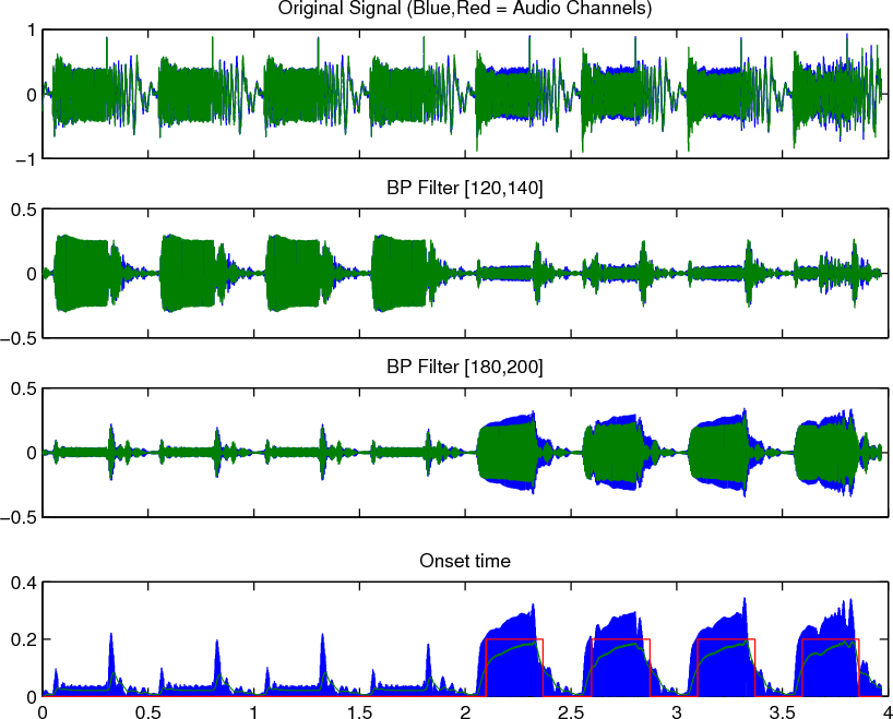
Detecting onset time and BP filtering:
Original Signal
[y,fs] = wavread('Brad_Sucks_-_Making_Me_Nervous_10s-18s.wav');
x=y(1:175e3,:);
t= (1:175e3)/fs;

subplot(411); plot(t,x); set(gca,'XTickLabels',[]);
title 'Original Signal (Blue,Red = Audio Channels)'

Wbp= [120 140]/(fs/2); %NOT HOW WE DEFINE w IN COURSE
[b,a] = cheby1(2,0.2,Wbp);
y1= filter(b,a,x);
subplot(412); plot(t,y1); set(gca,'XTickLabels',[]);
title 'BP Filter [120,140]'

Wbp= [180 200]/(fs/2);
[b,a] = cheby1(2,0.2,Wbp);
y2= filter(b,a,x);
subplot(413); plot(t,y2); set(gca,'XTickLabels',[]);
title 'BP Filter [180,200]'

z= abs(y2(:,1));
zf = filter(.001,[1,-.999],z);
zt = 0.2*(zf>.1);
subplot(414); plot(t,[z,zf,zt]); title 'Onset time'

Output:
  Output Image
|
|
Oct. 24
| |
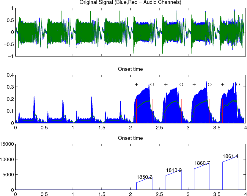
Detecting signal amplitude
Original Signal
[y,fs] = wavread('Brad_Sucks_-_Making_Me_Nervous_10s-18s.wav');
x=y(1:175e3,:);
t= (1:175e3)/fs;

subplot(311); plot(t,x); set(gca,'XTickLabels',[]);
title 'Original Signal (Blue,Red = Audio Channels)'

z= abs(y2(:,1));
zf = filter(.001,[1,-.999],z);

%SCHMITT TRIGGER
thresh = 0.1;
for i=1:length(zf)
  if zf(i) > thresh; thresh = 0.09; zt(i) = 1;end
  if zf(i) < thresh; thresh = 0.11; zt(i) = 0;end
end
subplot(312); plot(t,[z,zf,0.2*zt]); title 'Onset time'

startpts = find( diff(zt)>0 );
endpts   = find( diff(zt)<0 );

hold on;
plot(t(startpts),0.32,'k+');
plot(t(endpts),0.32,'ko');
hold off;

zs = filter(1,[1,-1],z);
subplot(313); plot(t,[zs.*zt]); title 'Amplitude'
for i=1:length(startpts)
  delta = zs(endpts(i)) - zs(startpts(i));
  text(t(startpts(i)), zs(endpts(i)), sprintf('%5.1f',delta));
end

Output:
  Output Image
|
|
Oct. 31
| |
Bandpass filter Design
[y,Fs] = wavread('Brad_Sucks_-_Making_Me_Nervous_10s-18s.wav');
x=y(1:175e3,1); t= (1:175e3)/Fs;

F0 = 200; f0 = F0/Fs;
Fc =  20; fc = Fc/Fs;
TBW = .001;
%Require 50dB, use Hamming
L = ceil(1.90/TBW);
W = hamming(2*L+1);

n=(-L:L)';
h_BP = 2*fc*sinc(2*fc*n) .* (2*cos(2*pi*f0*n));
subplot(311);
plot(n+L,h_BP,'k',n+L,h_BP.*W,'b');
xlim([0,2*L]);

subplot(312);
semilogy(linspace(0,Fs,2*L+1),abs(fft([h_BP,h_BP.*W])));
xlim([0,500]); ylim([1e-4,1]);

subplot(313);
plot(t,[x,3*filter(h_BP.*W,1,x)]);

Output:
  Output Image
|
|
Nov. 5
| |
Spectrogram
[y,Fs] = wavread('Brad_Sucks_-_Making_Me_Nervous_10s-18s.wav');
x=y(1:175e3,1); t= (1:175e3)/Fs; clf

axes('position',[0.04,0.68,0.92,0.28]);
specgram(x,64,Fs);
xlabel(''); set(gca,'Xticklabel',[]);
ylabel('N=64'); set(gca,'Yticklabel',[]); ylim([0,5e3]);

axes('position',[0.04,0.38,0.92,0.28]);
specgram(x,512,Fs);
xlabel(''); set(gca,'Xticklabel',[]);
ylabel('N=512'); set(gca,'Yticklabel',[]); ylim([0,5e3]);

axes('position',[0.04,0.08,0.92,0.28]);
specgram(x,4096,Fs);
ylabel('N=4096'); set(gca,'Yticklabel',[]); ylim([0,5e3]);
xlabel('Frequency (0-5kHz) vs Time (s)');

Output:
  Output Image
|
|
Nov. 26
| |
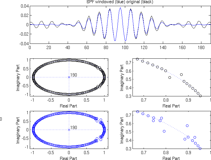
BPF and z-plane zeros
Fs = 44100; Fs = Fs/20; % Scale Fs (otherwise too many to view)

F0 = 200; f0 = F0/Fs;
Fc =  20; fc = Fc/Fs;
TBW = .02;
%Require 50dB, use Hamming
L = ceil(1.90/TBW);
W = hamming(2*L+1);

n=(-L:L)';
h_BP = 2*fc*sinc(2*fc*n) .* (2*cos(2*pi*f0*n));
h_BP_W = h_BP.*W;
subplot(311);
plot(n+L,h_BP,'k',n+L,h_BP_W,'b');
xlim([0,2*L]);
title 'BPF windowed (blue) original (black)'

subplot(323);
hh=zplane(h_BP', [1,zeros(1,2*L)]);
set(hh,'Color',[0,0,0]);
axis(1.1*[-1,1,-1,1]); axis normal

subplot(324);
hh=zplane(h_BP', [1,zeros(1,2*L)]);
set(hh,'Color',[0,0,0]);
axis([0.65,1.0,.3,.75]); axis normal

subplot(325);
zplane(h_BP_W', [1,zeros(1,2*L)]);
axis(1.1*[-1,1,-1,1]); axis normal

subplot(326);
zplane(h_BP_W', [1,zeros(1,2*L)]);
axis([0.65,1.0,.3,.75]); axis normal


Output:
  Output Image
|
|
Nov. 27
| |
Distortion effects
Common code to all distortion examples
[y,Fs] = wavread('Brad_Sucks_-_Making_Me_Nervous_10s-18s.wav');
ch1 = y(:,1)/2; ch2 = y(:,2)/2; time = (0:length(y)-1)/Fs;

original


Increase Stereo separation

% Increase stereo separation
chm = 0.5*[ch1+ch2];
chd = 0.5*[ch1 - ch2];
for sep = [0,1,2,4]
   out1 = chm + sep*chd;
   out2 = chm - sep*chd;

   fname = sprintf('stereo-sep%3.1f.wav',sep);
   wavwrite([out1,out2],Fs, fname);
end

Output:
original,
stereo-sep0.0.wav,
stereo-sep1.0.wav,
stereo-sep2.0.wav,
stereo-sep4.0.wav,


Adding reverb of different lengths

% reverb
for rev_len = [1000,3000,10000];
   fir = [1,zeros(1,rev_len-1)];
   RN = 20;
   fir(ceil(rev_len*rand(1,RN))) = 0.5*randn(1,RN);
   out1 = filter(fir,1,ch1)/2;
   out2 = filter(fir,1,ch2)/2;
   fname = sprintf('reverb-samp%4d.wav',rev_len);
   wavwrite([out1,out2],Fs, fname);
end

Output:
original,
reverb-samp1000.wav,
reverb-samp3000.wav,
reverb-samp10000.wav,


Non-linear distortion

cha = 0.5*[ch1+ch2];
for  distfac=[200,500];
   chf = cha*distfac;
   out = atan(chf);
   out = out/max(abs(out))*lim_chf; % set to original amplitude
   out = out + chr; % add in other frequencies
   fname = sprintf('nonlin=%3.1f.wav',distfac);
   wavwrite(out,Fs, fname);
end

Output:
original,
nonlin=200.0.wav,
nonlin=500.0.wav


Non-linear distortion in a Band-Pass filtered region.

F0 = 200; f0 = F0/Fs;
Fc =  50; fc = Fc/Fs;
TBW = .02;
%Require 50dB, use Hamming
L = ceil(1.90/TBW);
W = hamming(2*L+1);

n=(-L:L)';
h_BP = 2*fc*sinc(2*fc*n) .* (2*cos(2*pi*f0*n));
h_BP_W = h_BP.*W;
h_BS   = (n==0) - h_BP_W;

chf = filter(h_BP_W,1,cha); lim_chf = max(abs(chf));
chr = filter(h_BS  ,1,cha);

for  distfac=[200,500];
   chf = chf*distfac;
   out = atan(chf);
   out = out/max(abs(out))*lim_chf; % set to original amplitude
   out = out + chr; % add in other frequencies
   fname = sprintf('nonlin-cf=%3.1f.wav',distfac);
   wavwrite(out,Fs, fname);
end

Output:
original,
nonlin-cf=200.0.wav,
nonlin-cf=500.0.wav
|
Last Updated:
$Date: 2023/01/10 14:29:48 $
|
