EIDORS: Electrical Impedance Tomography and Diffuse Optical Tomography Reconstruction Software

Hosted by

Absolute and Difference solvers

Get data from the RPI tank phantom

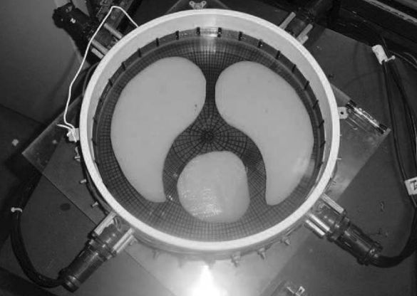
Figure: Figure: Phantom Image (from Isaacson, Mueller, Newell and Siltanen, IEEE Trans Med Imaging 23(7): 821-828, 2004)

Build a good FEM of the phantom

% RPI tank model $Id: rpi_data01.m 3790 2013-04-04 15:41:27Z aadler $

Nel= 32; %Number of elecs
Zc = .0001; % Contact impedance
curr = 20; % applied current mA


th= linspace(0,360,Nel+1)';th(1)=[];
els = [90-th]*[1,0]; % [radius (clockwise), z=0]
elec_sz = 1/6;
fmdl= ng_mk_cyl_models([0,1,0.1],els,[elec_sz,0,0.03]);

for i=1:Nel
   fmdl.electrode(i).z_contact= Zc;
end

% Trig stim patterns
th= linspace(0,2*pi,Nel+1)';th(1)=[];
for i=1:Nel-1;
   if i<=Nel/2;
      stim(i).stim_pattern = curr*cos(th*i);
   else;
      stim(i).stim_pattern = curr*sin(th*( i - Nel/2 ));
   end
   stim(i).meas_pattern= eye(Nel)-ones(Nel)/Nel;
   stim(i).stimulation = 'Amp';
end

fmdl.stimulation = stim;

clf; show_fem(fmdl,[0,1])

print_convert('rpi_data01a.png','-density 60');

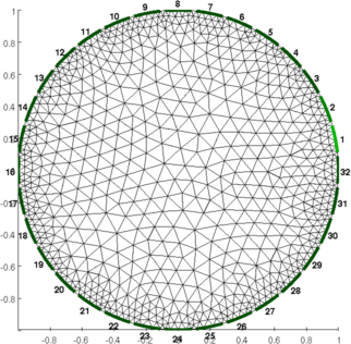
Figure: Figure: FEM phantom

Load and preprocess data

% load RPI tank data $Id: rpi_data02a.m 2236 2010-07-04 14:16:21Z aadler $

load Rensselaer_EIT_Phantom;
vh = real(ACT2006_homog);
vi = real(ACT2000_phant);

if 1
% Preprocessing data. We ensure that each voltage sequence sums to zero
  for i=0:30
    idx = 32*i + (1:32);
    vh(idx) = vh(idx) - mean(vh(idx));
    vi(idx) = vi(idx) - mean(vi(idx));
  end
end

Difference imaging

% RPI tank model $Id: rpi_data02b.m 3790 2013-04-04 15:41:27Z aadler $

% simple inverse model -> replace fields to match this model
imdl = mk_common_model('b2c2',32);
imdl.fwd_model = mdl_normalize(imdl.fwd_model, 0);

imdl.fwd_model.electrode = imdl.fwd_model.electrode([8:-1:1, 32:-1:9]);

imdl.fwd_model = rmfield(imdl.fwd_model,'meas_select');
imdl.fwd_model.stimulation = stim;
imdl.hyperparameter.value = 1.00;

% Reconstruct image
img = inv_solve(imdl, vh, vi);
img.calc_colours.cb_shrink_move = [0.5,0.8,0.02];
img.calc_colours.ref_level = 0;
clf; show_fem(img,[1,1]); axis off; axis image

print_convert('rpi_data02a.png','-density 60');

% RPI tank model $Id: rpi_data03.m 3790 2013-04-04 15:41:27Z aadler $

% simple inverse model -> replace fields to match this model
imdl.fwd_model = fmdl; 

img = inv_solve(imdl , vh, vi);
img.calc_colours.cb_shrink_move = [0.5,0.8,0.02];
img.calc_colours.ref_level = 0;
clf; show_fem(img,[1,1]); axis off; axis image

print_convert('rpi_data03a.png','-density 60');

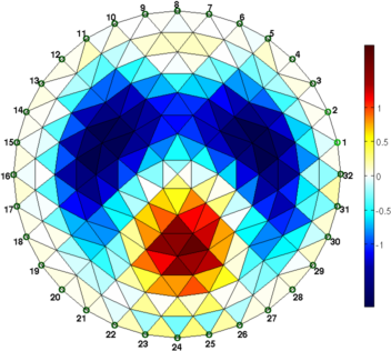
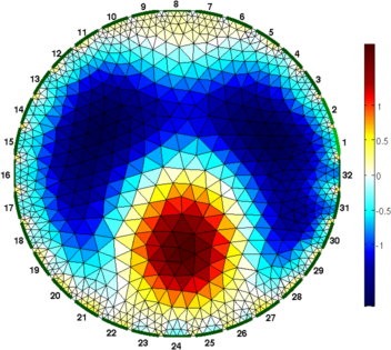
Figure: Figure: Differences images reconstructed of the phantom. For difference imaging, the simple model works surprisingly well.

Estimating actual conductivities

% RPI tank model $Id: rpi_data04.m 5509 2017-06-06 14:33:29Z aadler $

% In 3D, it's important to get the model diameter right, 2D is
imdl.fwd_model.nodes= imdl.fwd_model.nodes*15; % 30 cm diameter

% Estimate the background conductivity
imgs = mk_image(imdl);
vs = fwd_solve(imgs); vs = vs.meas;

pf = polyfit(vh,vs,1);

imdl.jacobian_bkgnd.value = pf(1)*imdl.jacobian_bkgnd.value;
imdl.hyperparameter.value = imdl.hyperparameter.value/pf(1)^2;

img = inv_solve(imdl, vh, vi);
img.calc_colours.cb_shrink_move = [0.5,0.8,0.02];
img.calc_colours.ref_level = 0;
clf; show_fem(img,[1,1]); axis off; axis image

print_convert('rpi_data04a.png','-density 60');

% Cheap static solver $Id: rpi_data05.m 3790 2013-04-04 15:41:27Z aadler $

% Do a diff solve with respect to simulated data
imgs = mk_image(imdl);
vs = fwd_solve(imgs); vs = vs.meas;


imdl.hyperparameter.value = 1.00;
img = inv_solve(imdl, vs, vi);
img.elem_data = pf(1) + img.elem_data*0.5;
img.calc_colours.cb_shrink_move = [0.5,0.8,0.02];
clf; show_fem(img,[1,1]); axis off; axis image

print_convert('rpi_data05a.png','-density 60');

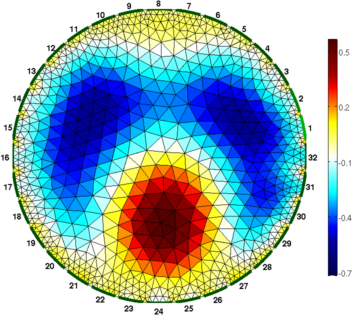
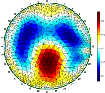
Figure: Difference (right) and one step absolute (left) images

Absolute solvers as a function of iteration

% Absolute reconstructions $Id: rpi_data06.m 5537 2017-06-14 12:49:20Z aadler $

imdl = mk_common_model('b2c2',32);
imdl.fwd_model = fmdl;
imdl.reconst_type = 'absolute';
imdl.hyperparameter.value = 2.0;
imdl.solve = @inv_solve_abs_GN;

for iter = [1,2,3, 5];
   imdl.inv_solve_gn.max_iterations = iter;
   img = inv_solve(imdl , vi);
   img.calc_colours.cb_shrink_move = [0.5,0.8,0.02];
   img.calc_colours.ref_level = 0.6;
   clf; show_fem(img,[1,1]); axis off; axis image

   print_convert(sprintf('rpi_data06%c.png', 'a'-1+iter),'-density 60');
end

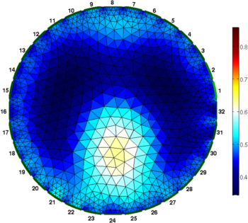
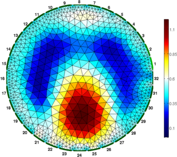
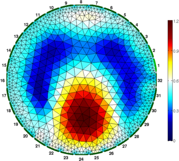
Figure: Gauss-Newton Absolute solver on conductivity at iterations (from left to right): 1, 3, 5

% Absolute reconstructions $Id: rpi_data07.m 4986 2015-05-11 20:09:28Z aadler $

imdl = mk_common_model('b2c2',32);
imdl.fwd_model = fmdl;
imdl.reconst_type = 'absolute';
imdl.hyperparameter.value = 2.0;
imdl.solve = @inv_solve_abs_CG;
imdl.inv_solve_abs_CG.elem_working = 'log_conductivity';
imdl.inv_solve_abs_CG.elem_output  =     'conductivity';

for iter = [1,2,3, 5];
   imdl.parameters.max_iterations = iter;
   img = inv_solve(imdl , vi);
   img.calc_colours.cb_shrink_move = [0.5,0.8,0.02];
   img.calc_colours.ref_level = 0.6;
   clf; show_fem(img,[1,1]); axis off; axis image

   print_convert(sprintf('rpi_data07%c.png', 'a'-1+iter),'-density 60');
end

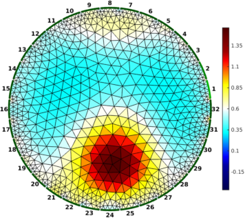
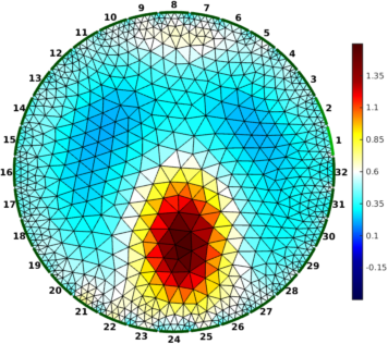
Figure: Conjugate-Gradient Absolute solver on log conductivity at iterations (from left to right): 1, 3, 5