EIDORS: Electrical Impedance Tomography and Diffuse Optical Tomography Reconstruction Software

Hosted by

GN reconstruction vs Backprojection

This tutorial explores the concept of reconstruction from electrical field projections, but does not implement the original backprojection algorithm.

The reconstruction matrix output by the original algorithm has been made available as part of EIDORS, here

Calculate the nodal voltage field

%$Id: backproj_solve01.m 4067 2013-05-26 20:17:46Z bgrychtol $
clf;
imdl= mk_common_model('c2c',16);

fmdl= imdl.fwd_model;
    ee= fmdl.elems';
    xx= reshape( fmdl.nodes(ee,1),3, []); 
    yy= reshape( fmdl.nodes(ee,2),3, []); 

for i=1:4
   if     i==1; stim= [0,1];
   elseif i==2; stim= [0,2];
   elseif i==3; stim= [0,4];
   elseif i==4; stim= [0,8];
   end

   fmdl.stimulation = mk_stim_patterns(16,1,stim,[0 1], {}, 1);
   img= mk_image(fmdl, 1);
   
   node_v= calc_all_node_voltages( img );
   zz{i}= reshape(     node_v(ee,4),3, []); 
end

for i=1:4
   subplot(2,4,i); cla
   patch(xx,yy,zz{i},zz{i}); view(0, 4); axis off
end

print_convert backproj_solve01a.png

for i=1:4
   subplot(2,4,i); cla
   patch(xx,yy,zz{i},zz{i}); view(0,34); axis off
end
print_convert backproj_solve01b.png

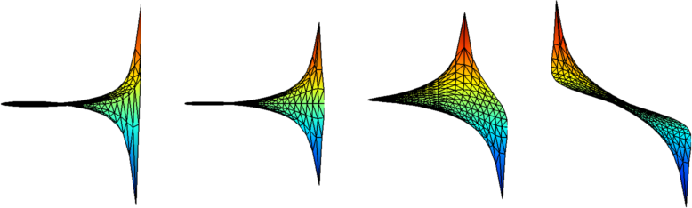
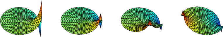
Figure: Nodal voltages in a mesh with different stimulation patterns. From Left to right: Adjacent stimulation ([0 1]), 45° stimulation ([0 2]), 90° stimulation ([0 4]), 180° stimulation ([0 8])

Calculate Equipotential lines

% $Id: backproj_solve02.m 3879 2013-04-18 09:26:22Z aadler $

clf; img = {};
% Solve voltage for 3 different models
for idx=1:3
  if     idx==1; mdltype= 'd2C2';
  elseif idx==2; mdltype= 'd2d3c';
  elseif idx==3; mdltype= 'd2T2';
  end

  pat = 4; % Stimulation pattern to show

  imdl= mk_common_model(mdltype,16);
  img{idx} = mk_image(imdl); 
  stim = mk_stim_patterns(16,1,'{ad}','{mono}',{'meas_current','rotate_meas'},-1);
  img{idx}.fwd_model.stimulation = stim(pat);
  img{idx}.fwd_solve.get_all_meas = 1;
end

% Show raw voltage pattern
for idx=1:3
  vh = fwd_solve(img{idx});
  imgn = rmfield(img{idx},'elem_data');
  imgn.node_data= vh.volt;
  subplot(2,3,idx); show_fem(imgn);
end
print_convert backproj_solve02a.png

% Calculate Equipotential lines
for idx=1:3
  vh = fwd_solve(img{idx});
  imgn = rmfield(img{idx},'elem_data');

  imgn.node_data= zeros(size(vh.volt,1),1);
  for v = 2:16
     imgn.node_data(vh.volt > vh.meas(v)) = v;
  end

  subplot(2,3,idx); show_fem(imgn);
end
print_convert backproj_solve02b.png

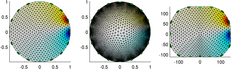
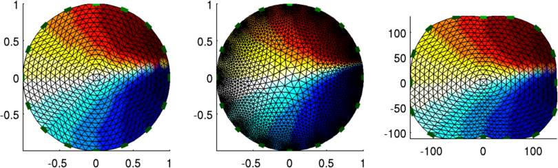
Figure: Equipotential lines for adjacent stimulation From Left to right: 1024 element circular mesh, 6746 element electrode refined element circular mesh, 1024 element mesh of human upper thorax

Create 2D Model and simulate measurements

% Compare 2D algorithms
% $Id: tutorial120a.m 3273 2012-06-30 18:00:35Z aadler $

imb=  mk_common_model('c2c',16);

e= size(imb.fwd_model.elems,1);
bkgnd= 1;

% Solve Homogeneous model
img= mk_image(imb.fwd_model, bkgnd);
vh= fwd_solve( img );

% Add Two triangular elements
img.elem_data([25,37,49:50,65:66,81:83,101:103,121:124])=bkgnd * 2;
img.elem_data([95,98:100,79,80,76,63,64,60,48,45,36,33,22])=bkgnd * 2;
vi= fwd_solve( img );

% Add -12dB SNR
vi_n= vi; 
nampl= std(vi.meas - vh.meas)*10^(-18/20);
vi_n.meas = vi.meas + nampl *randn(size(vi.meas));

show_fem(img);
axis square; axis off
print_convert('tutorial120a.png', '-density 60')

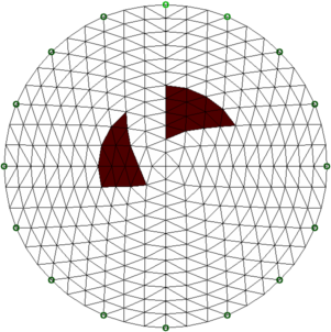
Figure: Sample image to test 2D image reconstruction algorithms

Image reconstruction with GN (NOSER) and Backprojection solvers

% $Id: backproj_solve03.m 4839 2015-03-30 07:44:50Z aadler $

tutorial120a; % get the model from a related tutorial

% Gauss Newton Solver
inv_GN= eidors_obj('inv_model','GN_solver','fwd_model', img.fwd_model);
inv_GN.reconst_type= 'difference';
inv_GN.solve= @inv_solve_diff_GN_one_step;
inv_GN.RtR_prior= @prior_noser;
inv_GN.jacobian_bkgnd.value= 1;
inv_GN.hyperparameter.value= 0.2;

imgr= inv_solve(inv_GN, vh,vi);
imgr.calc_colours.ref_level=0;
subplot(131); show_fem(imgr);
axis equal; axis off

% Backprojection Solver
inv_BP= eidors_obj('inv_model','BP_solver','fwd_model', img.fwd_model);
inv_BP.reconst_type= 'difference';
inv_BP.solve= @inv_solve_backproj;
inv_BP.inv_solve_backproj.type= 'naive';

imgr= inv_solve(inv_BP, vh,vi);
imgr.calc_colours.ref_level=0;
subplot(132); show_fem(imgr);
axis equal; axis off

inv_BP.inv_solve_backproj.type= 'simple_filter';

imgr= inv_solve(inv_BP, vh,vi);
imgr.calc_colours.ref_level=0;
subplot(133); show_fem(imgr);
axis equal; axis off

print_convert inv_solve_backproj03a.png

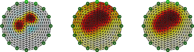
Figure: Reconstructions using: Left: GN Solver with NOSER Prior Middle: Naive Backprojection Right: Backprojection with a simple filter

GN vs Sheffield Backprojection

% Sheffield MKI backprojection $Id: backproj_solve04.m 4839 2015-03-30 07:44:50Z aadler $

% Gauss Newton Solvers
inv_mdl{1} = inv_GN;
inv_mdl{1}.hyperparameter.value= 0.2;
inv_mdl{2} = inv_GN;
inv_mdl{2}.hyperparameter.value= 0.5;
% Sheffield Backprojection solver
inv_mdl{3} = mk_common_gridmdl('backproj');

for loop=1:3
   imgr= inv_solve(inv_mdl{loop}, vh,vi);
   imgr.calc_colours.ref_level=0;
   subplot(1,3,loop); show_fem(imgr);
   axis equal; axis off
end

print_convert inv_solve_backproj04a.png

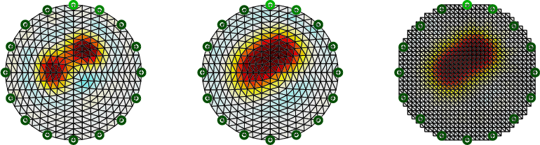
Figure: Reconstructions using: Left: GN Solver with NOSER Prior (small hyperparameter) Middle:GN Solver with NOSER Prior (larger hyperparameter) Right: Sheffield Mk I Backprojection