| Authors: | David C Barber,
Brian H Brown
|
|---|---|
| Date: | June 2008
|
| Brief Description: |
There are several different versions of the backprojection
algorithm in existence. The one made available here is
the version distributed with the Sheffield Mk I system,
and is very similar to the algorithm distributed with
the Göttingen Goe MF II EIT system. Almost all clinical
and experimental publications which mention "backprojection"
use the version of the algorithm provided here. The
paper which probably best describes this algorithm
is
Santosa, F. and Vogelius, M. (1990)
Backprojection algorithm for electrical
impedance imaging, SIAM J. Applied
Mathematics, 50:216−243.
|
| License: |
This matrix is copyright DC Barber and BH Brown at
University of Sheffield. It may be used free of
charge for research and non-commercial purposes.
Commercial applications require a licence from the
University of Sheffield.
|
| Attribution Requirement: |
Publications or presentations using these data should reference this publication:
D.C. Barber and B.H. Brown (1984),
Applied Potential Tomography,
J. Phys. E: Sci. Instrum., 17:723-733.
|
| Format: |
In order to save space, only 1/8 of the image and 1/2 (reciprocity
values) of the measurements are stored. In order to unpackage it,
the following code from mk_common_gridmdl
may be used:
[x,y]= meshgrid(1:16,1:16); % Take a slice ss1 = (y-x)>1 & (y-x)<15; sel1 = abs(x-y)>1 & abs(x-y)<15; [x,y]= meshgrid(-15.5:15.5,-15.5:15.5); ss2 = abs(x-y)<25 & abs(x+y)<25 & x<0 & y<0 & x>=y ; sel2 = abs(x-y)<25 & abs(x+y)<25; load Sheffield_Backproj_Matrix.mat BP = zeros(16^2, 32^2); BP(ss1,ss2) = Sheffield_Backproj_Matrix; BP = reshape(BP, 16,16,32,32); % Build up BP = BP + permute(BP, [2,1,3,4]); % Reciprocity el= 16:-1:1; BP= BP + BP(el,el,[32:-1:1],:); % FLIP LR el= [8:-1:1,16:-1:9]; BP= BP + BP(el,el,:,[32:-1:1]); % FLIP UD el= [12:-1:1,16:-1:13]; BP= BP + permute(BP(el,el,:,:), [1,2,4,3]); % Transpose RM= reshape(BP, 256, [])'; RM= RM(sel2,sel1); |
| Methods: |
|
| Data: | The Backprojection matrix is distributed
with EIDORS (version≥3.3) in the sample_data
directory.
|
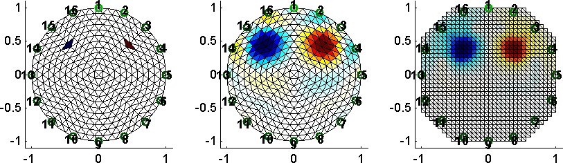
imdl= mk_common_model('c2c2',16);
img= calc_jacobian_bkgnd( imdl );
vh= fwd_solve(img);
img.elem_data([232,240])= 1.1;
img.elem_data([225,249])= 0.9;
vi= fwd_solve(img);
subplot(131); show_fem(img,[0,1,0]); axis square

img0 = inv_solve(imdl,vh,vi);
subplot(132); show_fem(img0,[0,1,0]); axis square

imdl=mk_common_gridmdl('backproj');
img1 = inv_solve(imdl,vh,vi);
subplot(133); show_fem(img1,[0,1,0]); axis square

print -dpng -r100 db_backproj_matrix01.png
 Last Modified: $Date: 2017-02-28 13:12:08 -0500 (Tue, 28 Feb 2017) $ by $Author: aadler $