EIDORS: Electrical Impedance Tomography and Diffuse Optical Tomography Reconstruction Software

Hosted by

Strange Effect: Conformal deformations of boundary shape

Create a simple model and deform it

% Linear model $Id: conformal1_01.m 3631 2012-11-18 18:34:04Z aadler $
xl=-3; xr= 3; yb=-15; yt= 15;
[x,y] = meshgrid( linspace(xl,xr,7), linspace(yb,yt,31) );
vtx= [y(:),x(:)];

elec_nodes{1}= [y(1,:);x(1,:)]';
elec_nodes{2}= [y(end,:);x(end,:)]';

z_contact= 0.01;
fmdl= mk_fmdl_from_nodes( vtx, elec_nodes, z_contact, 'sq_m1');
fmdl.stimulation(1).stimulation='Amp';
fmdl.stimulation(1).stim_pattern=[1;-1];
fmdl.stimulation(1).meas_pattern=[1,-1];

% Add non-conductive target
ctr = interp_mesh( fmdl,0); xctr= ctr(:,1); yctr= ctr(:,2);
img = mk_image( fmdl,  ones(length(xctr),1) );
img.elem_data( yctr>-3 & yctr<2 & xctr>8   & xctr<10 ) = 0.01;
img.elem_data( yctr> 0 & yctr<2 & xctr>-10 & xctr<10 ) = 0.01;


subplot(221)
show_fem(img); axis image

print_convert conformal1_01a.png '-density 125'



% Confromal deformation
z= fmdl.nodes(:,1) + 1i*fmdl.nodes(:,2);
z= exp((z-(20+80i))/100).*(z+20i).*(z-10i);
img2 = img; img2.fwd_model.nodes = [real(z), imag(z)];

show_fem(img2); axis image

print_convert conformal1_01b.png '-density 125'

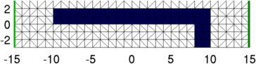
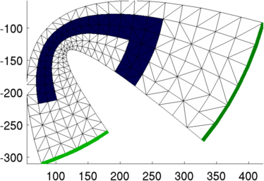
Figure: Rectangular model (Right) and the same model with a conformal deformation z_new= e^{.01(z-20-80i )}(z+20i)(z-10i) (left)

Solve the fwd problem on the flat and deformed model

% Voltage distribution $Id: conformal1_02.m 3215 2012-06-29 20:48:41Z aadler $

img.fwd_solve.get_all_meas = 1;
vv = fwd_solve(img);

imgv = rmfield(img,'elem_data');
imgv.node_data = vv.volt;

show_fem( imgv ); axis image

print_convert conformal1_02a.png '-density 125'

img2.fwd_solve.get_all_meas = 1;
vv = fwd_solve(img2);

imgv = rmfield(img2,'elem_data');
imgv.node_data = vv.volt;

show_fem( imgv ); axis image
print_convert conformal1_02b.png '-density 125'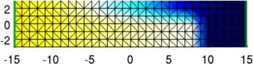

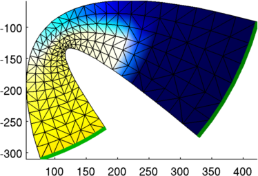
Figure: Voltage distribution in model (Right) and the same model with a conformal deformation z_new= e^{.01(z-20-80i )}(z+20i)(z-10i) (left)

% Voltage distribution $Id: conformal1_03.m 3634 2012-11-18 22:19:43Z aadler $

nodes = img.fwd_model.nodes; mn = min(nodes); mx= max(nodes);
img.fwd_model.mdl_slice_mapper.x_pts = linspace(mn(1),mx(1),50);
img.fwd_model.mdl_slice_mapper.y_pts = linspace(mn(2),mx(2),15);
img.calc_colours.clim = 5;

hh=show_fem(img); axis image;
set(hh,'EdgeColor',[0.5,0.5,0.5]);
hold on;
show_current( img); 
hold off;

print_convert conformal1_03a.png '-density 150'

nodes = img2.fwd_model.nodes; mn = min(nodes); mx= max(nodes);
img2.fwd_model.mdl_slice_mapper.x_pts = linspace(mn(1),mx(1),50);
img2.fwd_model.mdl_slice_mapper.y_pts = linspace(mn(2),mx(2),50);
img2.calc_colours.clim = 5;

hh= show_fem(img2); axis image;
set(hh,'EdgeColor',[0.5,0.5,0.5]);
hold on;
show_current( img2); 
hold off;

print_convert conformal1_03b.png '-density 125'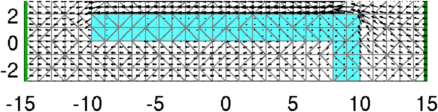

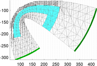
Figure: Current distribution in model (Right) and the same model with a conformal deformation z_new= e^{.01(z-20-80i )}(z+20i)(z-10i) (left)