EIDORS: Electrical Impedance Tomography and Diffuse Optical Tomography Reconstruction Software

Hosted by

Anisotroic deformations of medium shape

Create a simple resistor model and calculate current streamlines

% $Id: anisotropy1_01.m 4214 2013-06-17 12:39:48Z aadler $
xl=-3; xr= 3; yb=-15; yt= 15;
np= 35;
[x,y] = meshgrid( linspace(xr,xl,np), linspace(yb,yt,61) );
vtx= [y(:),x(:)];

for i=1:np
   elec_nodes{i   }= [y(1,i);x(1,i)]';
   elec_nodes{i+np}= [y(end,i);x(end,i)]';
end

z_contact= 1e5;
fmdl= mk_fmdl_from_nodes( vtx, elec_nodes, z_contact, 'sq_m1');
fmdl.stimulation(1).stimulation='Amp';
fmdl.stimulation(1).stim_pattern=[ones(np,1);-ones(np,1)];
fmdl.stimulation(1).meas_pattern=zeros(1,2*np); % don't care

% Add non-conductive target
ctr = interp_mesh( fmdl,0); xctr= ctr(:,1); yctr= ctr(:,2);
img = mk_image( fmdl,  ones(length(xctr),1) );



% Solve and add streamlines
img.fwd_solve.get_all_meas = 1;
vh = fwd_solve(img);

img.fwd_model.mdl_slice_mapper.npx = 200;
img.fwd_model.mdl_slice_mapper.npy = 100;
q = show_current(img,vh.volt);
hh=show_fem(img);
set(hh,'EdgeColor',[1,1,1]*.75);
hold on;
sy = linspace(-3,3,10); sx =  15+0*sy;
hh=streamline(q.xp,q.yp, q.xc, q.yc, sx,sy); set(hh,'Linewidth',2);
hold off;

axis image
axis([-16,16,-5,5]);
print_convert anisotropy1_01a.png '-density 125'

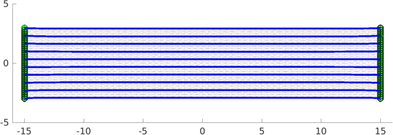
Figure: Rectangular model with current streamlines

Deform the model and recalculate streamlines

% Deformation $Id: anisotropy1_02.m 4214 2013-06-17 12:39:48Z aadler $
th = fmdl.nodes(:,1)/yt*(pi);
y = fmdl.nodes(:,2); y = y.*(th<=0) - y.*(th>0);
th = (th-pi/2).*(th<=0) + (pi/2-th).*(th>0);
[x,y] = pol2cart(th, y+4);
y = y+8.*(fmdl.nodes(:,1)<=0);
img2 = img; img2.fwd_model.nodes = [1.5*x, y];

img2.fwd_solve.get_all_meas = 1;
vh = fwd_solve(img2);

img_v = rmfield(img2,'elem_data');
img_v.node_data = vh.volt;
hh=show_fem(img_v);
set(hh,'EdgeColor',[1,1,1]*.75);

q=  show_current(img2,vh.volt);
hold on;
sy = -linspace(1.2,6.8,10); sx =  0*sy;
hh=streamline(q.xp,q.yp, q.xc, q.yc, sx,sy); set(hh,'Linewidth',2);
hold off;

axis image
print_convert anisotropy1_02a.png '-density 125'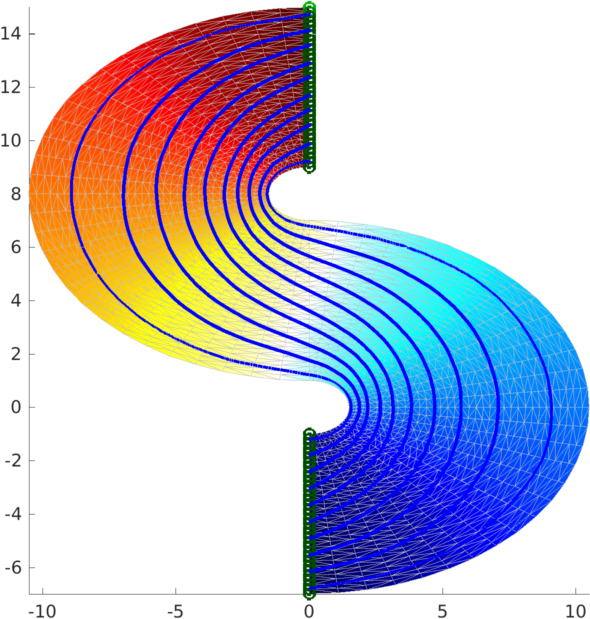

Figure: Deformed model with current streamlines

Create isotropic conductivity patterns and recalulate streamlines

% Deformation $Id: anisotropy1_03.m 4215 2013-06-17 12:55:18Z aadler $

xy = interp_mesh(img2.fwd_model);

% Create anisotropic conductivity.
clear conduct
   conduct(:,1,2,2) = abs(xy(:,1));
   conduct(:,1,1,1) = 1;
   conduct(:,1,1,2) = 0;
   conduct(:,1,2,1) = 0;
img2.elem_data = conduct;


img2.fwd_solve.get_all_meas = 1;
vh = fwd_solve(img2);

img_v.node_data = vh.volt;
hh=show_fem(img_v);
set(hh,'EdgeColor',[1,1,1]*.75);

q=  show_current(img2,vh.volt);
hold on;
sy =  linspace(1.2,6.8,10); sx =  0*sy;
hh=streamline(q.xp,q.yp, q.xc, q.yc, sx,sy); set(hh,'Linewidth',2);
hh=streamline(q.xp,q.yp,-q.xc,-q.yc, sx,sy); set(hh,'Linewidth',2);
hold off;

axis image
print_convert anisotropy1_03a.png '-density 125'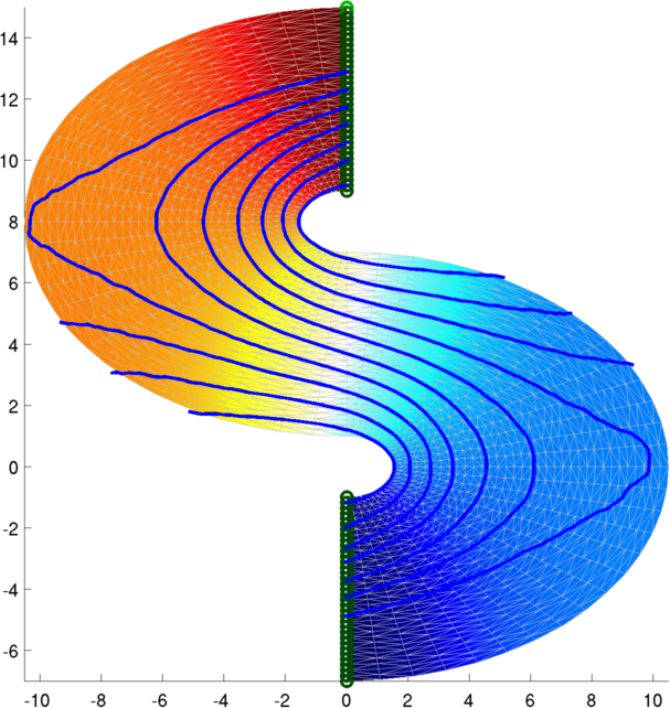

Figure: Deformed model with current streamlines