|
|
EIDORS: Electrical Impedance Tomography and Diffuse Optical Tomography Reconstruction Software |
|
EIDORS
(mirror) Main Documentation Tutorials − Image Reconst − Data Structures − Applications − FEM Modelling − GREIT − Old tutorials − Workshop Download Contrib Data GREIT Browse Docs Browse SVN News Mailing list (archive) FAQ Developer
Hosted by |
2D Geophysical models using square mesh elementsThis tutorial shows how a model can be built directly by specifying node locations and using the function mk_fmdl_from_nodes. Unfortunately, this technique cannot work in 3D, because the matlab delaunay function has bugs with regular meshes (which Mathworks acknowledges, but somehow doesn't feel it should fix − interesting behaviour for a company that claims to want leadership in mathematical computing ... don't worry, I'm not bitter, I only lost several days of my valuable time this way)Create fine mesh
% $Id: square_mesh01.m 2790 2011-07-14 22:32:12Z aadler $

z_contact= 0.01;
n_elec= 17;
nodes_per_elec= 5;
elec_width= 0.2;
elec_spacing= 1.0;

xllim=-12; xrlim= 12; ydepth=-15;
[x,y] = meshgrid( linspace(xllim,xrlim,49), linspace(ydepth,0,31) );
vtx= [x(:),y(:)];
% Refine points close to electrodes - don't worry if points overlap
[x,y] = meshgrid( -9:.25:9, -3:.25:0 );
vtx= [vtx; x(:),y(:)];

xgrid=  linspace(-elec_width/2, +elec_width/2, nodes_per_elec)';
x2grid= elec_width* [-5,-4,-3,3,4,5]'/4;
for i=1:n_elec
% Electrode centre
  x0= (i-1-(n_elec-1)/2)*elec_spacing;
  y0=0;
  elec_nodes{i}= [x0+ xgrid, y0+0*xgrid];
  vtx= [ vtx; ...
        [x0 + x2grid   ,  y0             + 0*x2grid];
        [x0 + xgrid*1.5,  y0-elec_width/2+ 0*xgrid];
        [x0 + x2grid*1.5, y0-elec_width/2+ 0*x2grid];
        [x0 + xgrid*2   , y0-elec_width  + 0*xgrid];
        [x0 + xgrid*2   , y0-elec_width*2+ 0*xgrid]];
end

fmdl= mk_fmdl_from_nodes( vtx, elec_nodes, z_contact, 'sq_m1');


subplot(121)
show_fem(fmdl); axis image
subplot(122)
show_fem(fmdl); axis image; axis([-2 2 -2.5 0.5]);

print_convert square_mesh01a.png '-density 175'
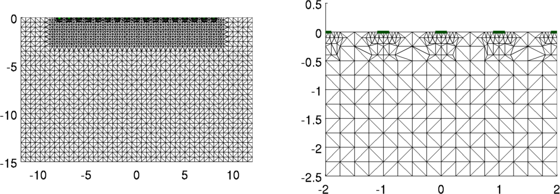 Figure:
Left: Fine mesh model with electrodes at surface
Right: close up view of mesh near electrodes Figure:
Left: Fine mesh model with electrodes at surface
Right: close up view of mesh near electrodes
Create Dual Mesh% Create and show square model $Id: square_mesh02.m 2790 2011-07-14 22:32:12Z aadler $ % Create square mesh model [cmdl,c2f]= mk_grid_model(fmdl, linspace(-8,8,17), linspace(-11.5,-0.5,13) ); clf; show_fem(fmdl); hold on; h= trimesh(cmdl.elems,cmdl.nodes(:,1),cmdl.nodes(:,2)); set(h,'Color',[0,0,1],'LineWidth',2); hold off axis image print_convert square_mesh02a.png 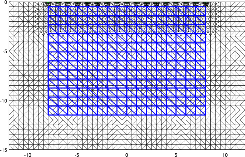 Figure:
Left: Uniform mesh density
Right: Mesh density refined going from surface to bottom Figure:
Left: Uniform mesh density
Right: Mesh density refined going from surface to bottom
Create Simulation Pattern
% simulate targets $Id: square_mesh03.m 3273 2012-06-30 18:00:35Z aadler $

fmdl.stimulation= mk_stim_patterns(length(elec_nodes), 1, '{ad}','{ad}', {}, 1);

img= mk_image(fmdl, 1);
vh= fwd_solve(img);

% interpolate onto mesh
xym= interp_mesh( fmdl, 3);
x_xym= xym(:,1,:); y_xym= xym(:,2,:);
% non-conductive target
ff  = (x_xym>-3) & (x_xym<-2) & (y_xym<-4) & (y_xym>-7);
img.elem_data= img.elem_data - 0.1*mean(ff,3);
% conductive target
ff  = (x_xym> 2) & (x_xym< 4) & (y_xym<-5) & (y_xym>-7);
img.elem_data= img.elem_data + 0.1*mean(ff,3);

% inhomogeneous image
vi= fwd_solve(img);

show_fem(img); axis image;
print_convert square_mesh03a.png
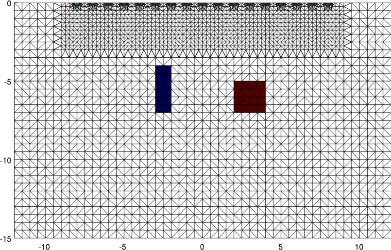 Figure:
Left: Uniform mesh density
Right: Mesh density refined going from surface to bottom Figure:
Left: Uniform mesh density
Right: Mesh density refined going from surface to bottom
Inverse Solution
% 2D solver $Id: square_mesh04.m 4839 2015-03-30 07:44:50Z aadler $

% Create a new inverse model, and set
% reconstruction model and fwd_model
imdl= mk_common_model('c2c2',16);
imdl.rec_model= cmdl;
imdl.fwd_model= fmdl;

c2f= mk_coarse_fine_mapping( fmdl, cmdl);
imdl.fwd_model.coarse2fine = c2f;
%imdl.RtR_prior = @prior_gaussian_HPF;
imdl.RtR_prior = @prior_noser;
imdl.prior_use_fwd_not_rec = 1;
imdl.prior_noser.exponent= 0.5;
imdl.solve = @inv_solve_diff_GN_one_step;
imdl.hyperparameter.value= 0.05;

imgs= inv_solve(imdl, vh, vi);

show_fem(fmdl); ax= axis;
hold on
show_fem(imgs);
hold on;
h= trimesh(cmdl.elems,cmdl.nodes(:,1),cmdl.nodes(:,2));
set(h,'Color',[0,0,1]);
hold off
hold off
axis(ax); axis image
print_convert square_mesh04a.png
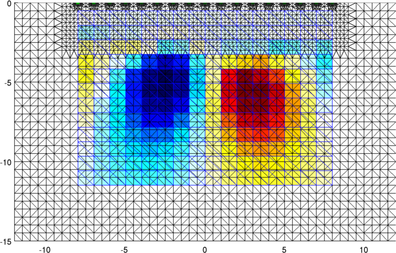 Figure:
Left: Uniform mesh density
Right: Mesh density refined going from surface to bottom Figure:
Left: Uniform mesh density
Right: Mesh density refined going from surface to bottom
Internal ElectrodesIn order to place internal electrodes, we cannot use the complete electrode model, instead, we place point electrodes as follows.
% $Id: square_mesh05.m 3097 2012-06-08 14:07:14Z bgrychtol $

z_contact= 0.01;
nodes_per_elec= 5;
n_elec=17;
elec_width= 0.2;
elec_spacing= 1.0;

xllim=-12; xrlim= 12; ydepth=-15;
[x,y] = meshgrid( linspace(xllim,xrlim,49), linspace(ydepth,0,31) );
vtx= [x(:),y(:)];
% Refine points close to electrodes - don't worry if points overlap
[x,y] = meshgrid( -9:.25:9, -3:.25:0 );
vtx= [vtx; x(:),y(:)];
[x,y] = meshgrid( -9:.25:9, -15:.25:-11 );
vtx= [vtx; x(:),y(:)];

xgrid=  linspace(-elec_width/2, +elec_width/2, nodes_per_elec)';
x2grid= elec_width* [-5,-4,-3,3,4,5]'/4;
for i=1:n_elec
  x0= (i-1-(n_elec-1)/2)*elec_spacing;

% Top electrode
  y0  = zeros(size(xgrid));
  y0_2= zeros(size(x2grid));
% elec_nodes{2*i-1}= [x0+ xgrid, y0];
  elec_nodes{2*i-1}= [x0, 0];
  vtx= [ vtx; ...
        [x0 + x2grid    , y0_2              ];
        [x0 + xgrid*1.5 , y0  - elec_width/2];
        [x0 + x2grid*1.5, y0_2- elec_width/2];
        [x0 + xgrid*2   , y0  - elec_width  ];
        [x0 + xgrid*2   , y0  - elec_width*2]];

% Bottom electrode
  y0  = -13*ones(size(xgrid));
  y0_2= -13*ones(size(x2grid));
  elec_nodes{2*i}= [x0,-13]; % Only point electrodes insidq
  vtx= [ vtx; ...
        [x0 + x2grid    , y0_2              ];
        [x0 + xgrid*1.5 , y0  - elec_width/2];
        [x0 + x2grid*1.5, y0_2- elec_width/2];
        [x0 + xgrid*1.5 , y0  + elec_width/2];
        [x0 + x2grid*1.5, y0_2+ elec_width/2];];
end

fmdl= mk_fmdl_from_nodes( vtx, elec_nodes, z_contact, 'sq_m1');
fmdl.solve=@fwd_solve_1st_order;
fmdl.system_mat=@system_mat_1st_order;
fmdl.jacobian=@jacobian_adjoint;


subplot(121)
show_fem(fmdl); axis image
subplot(122)
show_fem(fmdl); axis image; axis([-2 2 -14 -12]);

print_convert square_mesh05a.png
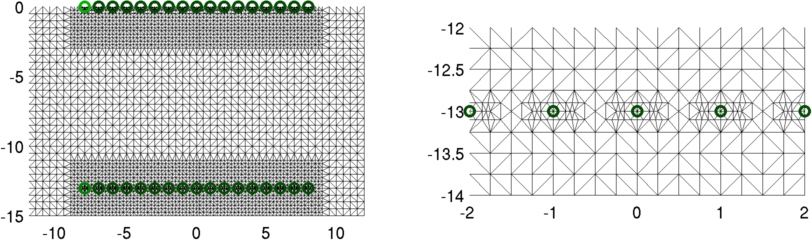 Figure:
Left: Uniform mesh density
Right: Mesh density refined going from surface to bottom Figure:
Left: Uniform mesh density
Right: Mesh density refined going from surface to bottom
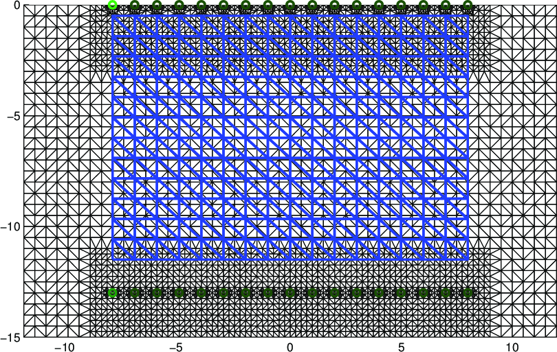 Figure:
Left: Uniform mesh density
Right: Mesh density refined going from surface to bottom Figure:
Left: Uniform mesh density
Right: Mesh density refined going from surface to bottom
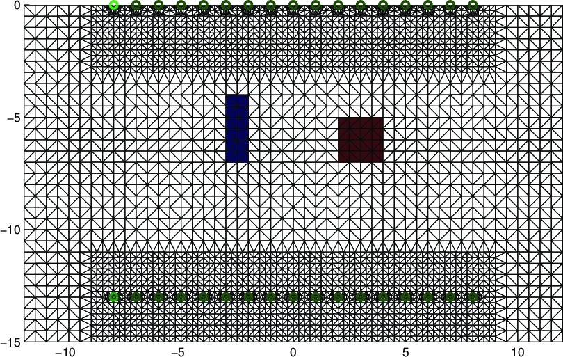 Figure:
Left: Uniform mesh density
Right: Mesh density refined going from surface to bottom Figure:
Left: Uniform mesh density
Right: Mesh density refined going from surface to bottom
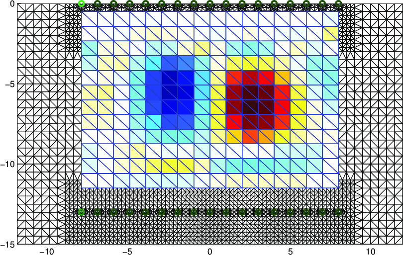 Figure:
Left: Uniform mesh density
Right: Mesh density refined going from surface to bottom Figure:
Left: Uniform mesh density
Right: Mesh density refined going from surface to bottom
|
Last Modified: $Date: 2017-02-28 13:12:08 -0500 (Tue, 28 Feb 2017) $ by $Author: aadler $