EIDORS: Electrical Impedance Tomography and Diffuse Optical Tomography Reconstruction Software

Hosted by

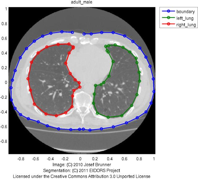
Modeling EIT current flow in a human thorax model

Load thorax shape and identify contours

load CT1.mat
img = flipdim(imread('thorax-mdl.jpg'),1); %Keep up direction
imagesc(img);
colormap(gray(256)); set(gca,'YDir','normal');

hold on;
plot(thorax(:,1),thorax(:,2),'b','LineWidth',2);
plot(rlung(:,1),rlung(:,2),'b','LineWidth',2);
plot(llung(:,1),llung(:,2),'b','LineWidth',2);
hold off

subplot(221); axis off; axis equal
print_convert thoraxmdl01a.jpg

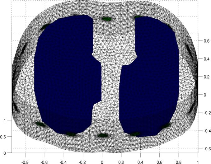
Use Netgen to build a FEM model of the thorax

f = 100;
[fmdl, mat_idx] = ng_mk_extruded_model({2,{thorax/f,rlung/f,llung/f},[4,50],.1},[16,1.00,1],[.1,0,.05]);
fmdl.nodes = fmdl.nodes*f;
[stim,meas_sel] = mk_stim_patterns(16,1,[0,1],[0,1],{'no_meas_current'}, 1);
fmdl.stimulation = stim;

img=mk_image(fmdl,1);
img.elem_data(mat_idx{2})= 0.3; % rlung
img.elem_data(mat_idx{3})= 0.3; % llung

clf; show_fem(img); view(0,70);
print_convert thoraxmdl02a.jpg

Voltage and Current Distribution in a slice

img_v = img;
% Stimulate between elecs 16 and 5 to get more interesting pattern
img_v.fwd_model.stimulation(1).stim_pattern = sparse([16;5],1,[1,-1],16,1);
img_v.fwd_solve.get_all_meas = 1;
vh = fwd_solve(img_v);

img_v = rmfield(img, 'elem_data');
img_v.node_data = vh.volt(:,1);
img_v.calc_colours.npoints = 128;

subplot(221);
show_slices(img_v,[inf,inf,1.0]); axis off; axis equal
print_convert thoraxmdl03a.jpg

img_v = img;
img_v.fwd_model.mdl_slice_mapper.npx = 64;
img_v.fwd_model.mdl_slice_mapper.npy = 64;
img_v.fwd_model.mdl_slice_mapper.level = [inf,inf,1.0];
show_current(img_v, vh.volt(:,1));

axis tight; axis image; ylim([50,450]); axis off
print_convert thoraxmdl04a.jpg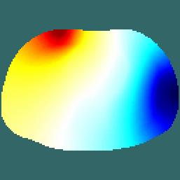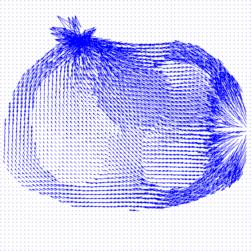

Left Voltage distribution and Right Current distribution in slices at z= 1.0.

Current streamlines and the original image

img_v.fwd_model.mdl_slice_mapper.npx = 1000;
img_v.fwd_model.mdl_slice_mapper.npy = 1000;
img_v.fwd_model.mdl_slice_mapper.level = [inf,inf,1.0];

% Calculate at high resolution
 q = show_current(img_v, vh.volt(:,1));

imgt= flipdim(imread('thorax-mdl.jpg'),1); imagesc(imgt);
colormap(gray(256)); set(gca,'YDir','normal');

sx = 250 - linspace(-130,130,15)';
sy = 250 + linspace(-130,130,15)';

hh=streamline(q.xp,q.yp, q.xc, q.yc,sx,sy); set(hh,'Linewidth',2);
hh=streamline(q.xp,q.yp,-q.xc,-q.yc,sx,sy); set(hh,'Linewidth',2);

axis equal; axis tight; axis off; print_convert thoraxmdl05a.jpg

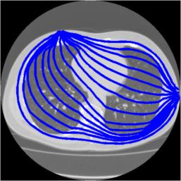
Stream lines through z= 1.0. The path of the streamslines is limited by the density of the underlying FEM. With a finer mesh FEM, it would be possible to calculate streamlines that do not display path irregularities.

Add Equipotential lines to the original image

img_v = img;
% Stimulate between elecs 16 and 5 to get more interesting pattern
img_v.fwd_solve.get_all_meas = 1;
vh = fwd_solve(img_v);

img_v = rmfield(img, 'elem_data');
img_v.node_data = vh.volt(:,08);
img_v.calc_colours.npoints = 256;
imgs = calc_slices(img_v,[inf,inf,1.0]);


clf
imagesc(imgt); colormap(gray(256)); set(gca,'YDir','normal');
hh=streamline(q.xp,q.yp, q.xc, q.yc,sx,sy); set(hh,'Linewidth',2);
hh=streamline(q.xp,q.yp,-q.xc,-q.yc,sx,sy); set(hh,'Linewidth',2);

[x,y] = meshgrid( linspace(2,size(imgt,1)-1,size(imgs,1)), ...
                  linspace(size(imgt,2)-1,2,size(imgs,2)) );
hold on;
hh=contour(x,y,imgs,20);
hh= findobj('Type','patch'); set(hh,'LineWidth',2)

hold off; axis off; axis equal; ylim([50,450]);
print_convert thoraxmdl06a.jpg

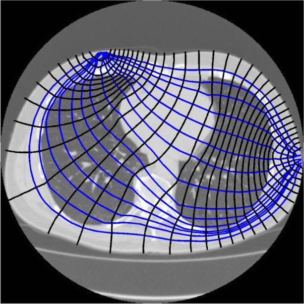
Stream lines and equipotiential through z= 1.0.