EIDORS: Electrical Impedance Tomography and Diffuse Optical Tomography Reconstruction Software

Hosted by

Using EIDORS to image geophysics

Borehole model

• Anneau1_Decembre2004_wen32_1.m
• Anneau1_Janvier2005_wen64_1.m
• Anneau1_Juillet2004_wen32_1.m
• dg_calc_jacobian.m
• dg_calc_system_mat.m
• dg_downhill_simplex_nr.m
• dg_fwd_parameters.m
• dg_fwd_solve.m
• dg_gallery_penalty_simplex.m
• dg_show_gallery_models.m
• Electrode_Positions_Ring1_EZG04.m
• elems_2Dto3D.m
• gallery_gradient.m
• lance_inversions_MontTerri.m
• mk_2Dto3D_mapping.m
• mk_Coarse2DtoFine3D_mapping.m
• mk_data_tomel.m
• mk_gallery.m
• mk_Pilot2DtoFine3D_mapping.m
• mk_stim_patterns_tomel.m

Create 3D FEM model of the gallery and load homogeneous model

% Create 3D FEM model of the gallery
% $Id: tutorial410a.m 2343 2010-11-03 17:47:50Z dgibert $
n_rings= 9;
factor= 2;
levels= [-6 -4 -2.5 -1.5 -1 -0.5 -0.25 0 0.25 0.5 1 1.5 2.5 4 6];

Electrode_Positions_Ring1_EZG04;
elec_posn= EZG04_Ring1;

Anneau1_Juillet2004_wen32_1;
data_tomel= Data_Ring1_July2004_Wen32_1;
real_data= mk_data_tomel(data_tomel,'Mont-Terri data','Wenner protocol');

gallery_3D_fwd = mk_gallery(elec_posn,data_tomel,n_rings,factor,levels);
gallery_3D_fwd.solve = 'aa_fwd_solve';
gallery_3D_fwd.system_mat = 'aa_calc_system_mat';
gallery_3D_fwd.jacobian = 'aa_calc_jacobian';


subplot(121)
show_fem(gallery_3D_fwd); axis square; view(0.,15.);
subplot(122)
show_fem(gallery_3D_fwd); axis square; view(0.,75);
%print -r100 -dpng tutorial410a.png;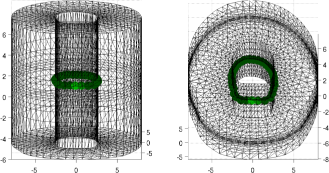

Figure: 3D FEM of gallery from two viewing angles

Create forward model. Calculate the difference (residual) between the gallery data and a homogeneous forward model.

% Reconstruct data on Gallery
% $Id: tutorial410b.m 2682 2011-07-13 08:20:30Z bgrychtol $

% homogeneous starting model
background_resistivity= 15.0; % Unit is Ohm.m
background_conductivity= 1./background_resistivity;

gallery_3D_img= eidors_obj('image',gallery_3D_fwd.name);
gallery_3D_img.fwd_model= gallery_3D_fwd;
gallery_3D_img.elem_data= background_conductivity * ...
   ones(size(gallery_3D_img.fwd_model.elems,1),1);

% build the parameter-to-elements mapping
%USE: sparse pilot-point parameterization
sparsity = 1;
gallery_3D_img= mk_Pilot2DtoFine3D_mapping(gallery_3D_img,sparsity);
gallery_3D_img.fwd_model.coarse2fine = kron(ones(42,1), speye(1024));

gallery_3D_img.rec_model.type = 'fwd_model';
gallery_3D_img.rec_model.name = '2d';
gallery_3D_img.rec_model.elems = gallery_3D_img.fwd_model.misc.model2d.elems;
gallery_3D_img.rec_model.nodes = gallery_3D_img.fwd_model.misc.model2d.nodes;

%disp(['Computing the CC and SS matrices = ' gallery_3D_img.fwd_model.misc.compute_CCandSS]);
%[ref_data,gallery_3D_img]= aa_fwd_solve(gallery_3D_img);
[ref_data]= fwd_solve(gallery_3D_img);
residuals= real_data.meas-ref_data.meas;

%% plot the data
subplot(211);
plot([ref_data.meas,real_data.meas]);
%print -r75 -dpng tutorial410b.png;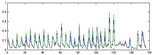

Figure: Electrode data: blue simulation, green measurement

Reconstruct image and show residual.

% Reconstruct data on Gallery
% $Id: tutorial410c.m 2343 2010-11-03 17:47:50Z dgibert $

n_iter=2;

gallery_3D_img.fwd_model.misc.compute_CCandSS='n';
for k= 1:n_iter
    eidors_msg('Iteration number %d',k,1);
    jacobian = calc_jacobian(gallery_3D_img);
    ref_data= fwd_solve(gallery_3D_img);
    residuals= real_data.meas-ref_data.meas;
    svj= svd(jacobian);
    % compute pseudo-inverse using only the largest singular values
    delta_params= pinv(jacobian,svj(1)/20.)*residuals;
    delta_params= delta_params.*gallery_3D_img.params_mapping.perturb;
    gallery_3D_img.params_mapping.params= gallery_3D_img.params_mapping.params + delta_params;
end

%% Solve final model and display results
ref_data= fwd_solve(gallery_3D_img);

subplot(211)
plot([ref_data.meas,real_data.meas]);
%print -r75 -dpng tutorial410c.png;

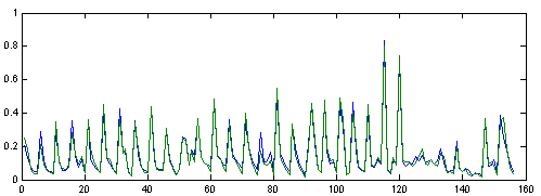
Figure: Electrode data: blue simulation, green measurement

Show reconstructed images

% Show images $Id: tutorial410d.m 2341 2010-11-03 15:35:00Z dgibert $

subplot(121)
axis square; view(30.,80.);
show_fem(gallery_3D_img);

subplot(122)
gallery_3D_resist= gallery_3D_img; % Create resistivity image
gallery_3D_resist.elem_data= 1./gallery_3D_img.elem_data;
show_slices(gallery_3D_resist,[inf,inf,0]);

%print -r125 -dpng tutorial410d.png;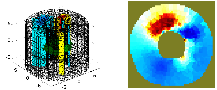

Figure: Reconstructed images: right: 3D, left: slice through centre