EIDORS: Electrical Impedance Tomography and Diffuse Optical Tomography Reconstruction Software

Hosted by

Create geophysical stimulation patterns and draw the corresponding pseudo-sections

In order to evaluate fastly the data quality, geophysicists usually represent pseudo-sections that allow a fast visualisation of the raw data. Pseudo-sections may also represent the residuals after the data inversion and so illustrate the repartition of fit quality. The show_pseudosection function allows such representation.

This tutorial gives an exemple of the two EIDORS functions constructed to create geophysical protocols and represent data in pseudo-sections.

Create 3D FEM model for a horizontal profile

% Forward Model
shape_str = ['solid top    = plane(0,0,0;0,0,1);\n' ...
             'solid mainobj= top and orthobrick(-100,-100,-200;410,100,0) -maxh=50.0;\n'];
n_elec= 54; 
e0 = linspace(0,310,n_elec)';
elec_pos = [e0,0*e0,0*e0,0*e0,0*e0,1+0*e0];
elec_shape= [0.005,0,1];
elec_obj = 'top';
fmdl = ng_mk_gen_models(shape_str, elec_pos, elec_shape, elec_obj);

% homogeneous conductivity of 0.1 Sm and insert a conductive sphere
img = mk_image(fmdl,0.1 + mk_c2f_circ_mapping(fmdl,[100;0;-50;20])*100);

hh= show_fem(img); view(-28,22); set(hh,'LineWidth',1);
print_convert stimPatt_PseudoSec01.png '-density 75'

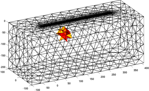
Figure: Forward model for which to calculate

Create a stimulation pattern with a Wenner protocol and show the pseudo-section

% Construct the Wenner stimulation pattern
img.fwd_model.stimulation= stim_pattern_geophys( n_elec, 'Wenner', {'spacings', 1:32} );

% Use apparent_resistivity
img.fwd_model.jacobian = @jacobian_apparent_resistivity;
img.fwd_model.solve    = @fwd_solve_apparent_resistivity;

% Solve the forward problem
dd  = fwd_solve(img);

% Show the pseudo-section of the apparent resistivity
show_pseudosection( img.fwd_model, dd.meas);
print_convert stimPatt_PseudoSec02.png '-density 100'

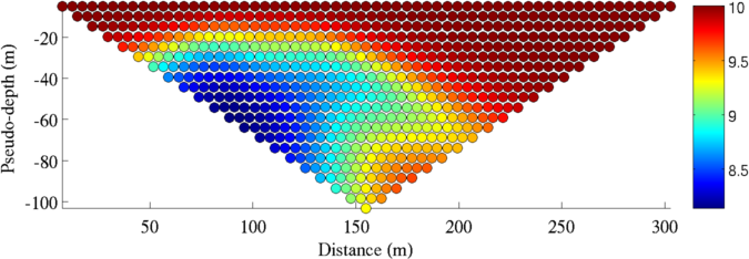
Figure: Pseudo-section for a horizontal profile using a Wenner protocol.

Create a stimulation pattern with a Schlumberger protocol and show the pseudo-section

% Construct the Schlumberger stimulation pattern
spacing= [1 1 1 2 3 4 6 8 8 11 12 14 17]; 		% Spacing between electrodes (usually called the "a" parameter)
multiples= [1 2 3 2 5/3 6/4 7/6 1 10/8 1 13/12 15/14 1];% Multiples (usually called the "n" parameter)
img.fwd_model.stimulation= stim_pattern_geophys( n_elec, 'Schlumberger', {'spacings', spacing,'multiples',multiples} );

% Solve the forward problem
dd  = fwd_solve(img);

% Show the pseudo-section of the apparent resistivity
show_pseudosection( img.fwd_model, dd.meas);
print_convert stimPatt_PseudoSec03.png '-density 100'

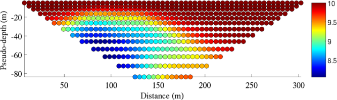
Figure: Pseudo-section for a horizontal profile using a Schlumberger protocol.

Create a stimulation pattern with a Dipole-dipole protocol and show the pseudo-section

% Construct the Dipole-dipole stimulation pattern
spacing= [1 1 1 2 3 3 4 4 5 6 6 7 8 8 9 10 10 11 12 12 13 14 14 15 16 17]; % Spacing between electrodes (usually called the "a" parameter)
multiples= [1 2 3 2 1 5/3 1 2  1 1 7/6 1 1 10/8 1 1 12/10 1 1 13/12 1 1 15/14 1 1 1]; % Multiples (usually called the "n" parameter)
img.fwd_model.stimulation= stim_pattern_geophys( n_elec, 'DipoleDipole', {'spacings', spacing,'multiples',multiples} );


% Solve the forward problem
dd  = fwd_solve(img);

% Show the pseudo-section of the apparent resistivity
show_pseudosection( img.fwd_model, dd.meas);
print_convert stimPatt_PseudoSec04.png '-density 100'

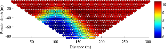
Figure: Pseudo-section for a horizontal profile using a Dipole-dipole protocol.

Case of borehole measurements (or any vertical acquisition setup)

% Forward Model including a borehole

borehole_diameter= 0.1;
n_elec= 32;
e0 = -linspace(0.5,5,n_elec)';
elec_pos = [0*e0,0*e0+borehole_diameter,e0,0*e0,1+0*e0,0*e0];
elec_shape= [0.04 0.02 0.1];

incyl = sprintf('cylinder (0,0,0; 0,0,-6;%f)',borehole_diameter); % Borehole
farcyl= sprintf('cylinder (0,0,0; 0,0,-15;10)'); % Medium surrounding the borehole
shape_str = ['solid incyl  = ',incyl,' -maxh=0.1 ; \n', ...
             'solid farcyl = ',farcyl,' -maxh=10 ; \n', ...
             'solid pli1   =  plane(0,0,0;0,0,1);\n' ...
             'solid pli2   =  plane(0,0,-6; 0,0,-1);\n' ...
             'solid plu1   =  plane(0,0,0;0,0,1);\n' ...
             'solid plu2   =  plane(0,0,-15; 0,0,-1);\n' ...
             'solid innerobj= pli1 and pli2 and incyl;\n', ...
             'solid mainobj= plu1 and plu2 and farcyl and not innerobj;\n'];
clear elec_obj
for i=1:size(e0,1) ;  elec_obj{i} = 'incyl';end
[fmdl,mat_idx] = ng_mk_gen_models(shape_str, elec_pos, elec_shape, elec_obj);


% Construct the Wenner stimulation pattern
fmdl.stimulation= stim_pattern_geophys( n_elec, 'Wenner', {'spacings', 1:25} );

% Use apparent_resistivity
fmdl.jacobian = @jacobian_apparent_resistivity;
fmdl.solve    = @fwd_solve_apparent_resistivity;


% Construct a model with a homogeneous conductivity of 0.1 Sm and insert a conductive sphere
img = mk_image(fmdl,0+ mk_c2f_circ_mapping(fmdl,[0;0.7;-3;0.3])*100);
img.elem_data(img.elem_data==0)= 0.1;
show_fem(img);
print_convert stimPatt_PseudoSec05_1.png '-density 75'
 
% Solve the forward problem
dd  = fwd_solve(img);

% Show the pseudo-section of the apparent resistivity
fmdl.show_pseudosection.orientation = 'vertical';
show_pseudosection( fmdl, dd.meas);
print_convert stimPatt_PseudoSec05_2.png '-density 75'

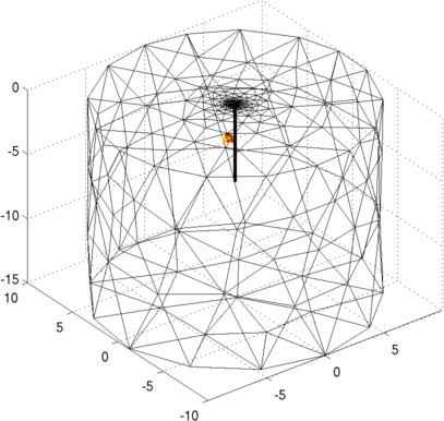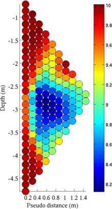
Figure: Forward model including a borehole and pseudo-section for a vertical profile using a Wenner protocol.

Case of circumferential measurements around a circular object (rock sample, human, tree...)

% Forward Model of a cylindrical object
n_elec= 32;
ring_vert_pos = [0.5]; 
fmdl= ng_mk_cyl_models([1,0.3,0.05],[n_elec,ring_vert_pos],[0.02,0.05,0.02]);


% Construct the Wenner stimulation pattern
fmdl.stimulation= stim_pattern_geophys( n_elec, 'Wenner', {'spacings', 1:7,'circumferential_meas',1} );

% Use apparent_resistivity
fmdl.jacobian = @jacobian_apparent_resistivity;
fmdl.solve    = @fwd_solve_apparent_resistivity;

% Construct a model with a homogeneous conductivity of 0.1 Sm and insert a conductive sphere
img = mk_image(fmdl,0.1+ mk_c2f_circ_mapping(fmdl,[0;0.10;0.5;0.1])*100);
show_fem(img);
print_convert stimPatt_PseudoSec06_1.png '-density 75'
 
% Solve the forward problem
dd  = fwd_solve(img);

% Show the pseudo-section of the apparent resistivity
fmdl.show_pseudosection.orientation = 'CircularInside';
show_pseudosection( fmdl, dd.meas);
print_convert stimPatt_PseudoSec06_2.png '-density 75'

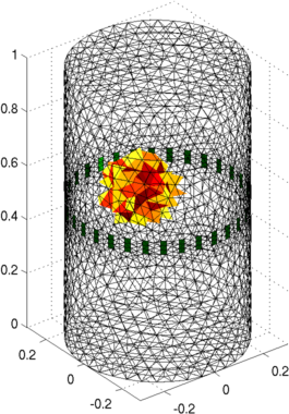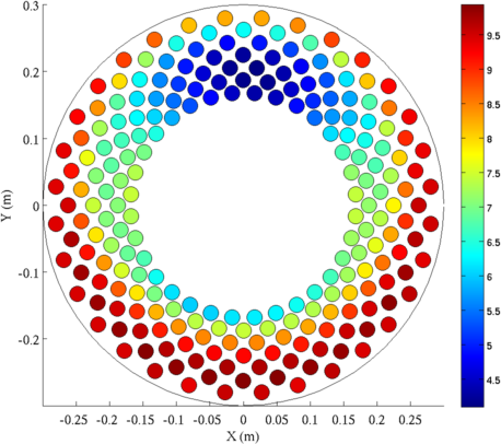
Figure: Forward model of a cylindrical obect and pseudo-section for circumferential inward measurements using a Wenner protocol.

Case of circumferential measurements around a cavity (gallery)

% Forward Model of a cylindrical object
% Create 3D model of a tunnel $Id: stimPatt_PseudoSec07.m 3902 2013-04-18 17:59:23Z aadler $
n_elec = 32;
shape_str = ['solid incyl  = cylinder (0,0,0; 1,0,0; 1) -maxh=1.0; \n', ...
    'solid farcyl = cylinder (0,0,0; 1,0,0; 5) -maxh=5.0; \n' ...
    'solid pl1    =  plane(-5,0,0;-1,0,0);\n' ...
    'solid pl2    =  plane(5,0,0; 1,0,0);\n' ...
    'solid mainobj= pl1 and pl2 and farcyl and not incyl;\n'];
th= linspace(0,2*pi,n_elec+1)'; th(end)=[];
cth= cos(th); sth=sin(th); zth= zeros(size(th));
elec_pos = [zth, cth, sth, zth cth, sth];
elec_shape= 0.01;
elec_obj = 'incyl';
fmdl = ng_mk_gen_models(shape_str, elec_pos, elec_shape, elec_obj);


% Construct the Wenner stimulation pattern
fmdl.stimulation= stim_pattern_geophys( n_elec, 'Wenner', {'spacings', 1:6,'circumferential_meas',1} );

% Use apparent_resistivity
fmdl.jacobian = @jacobian_apparent_resistivity;
fmdl.solve    = @fwd_solve_apparent_resistivity;

% Construct a model with a homogeneous conductivity of 0.1 Sm and insert a conductive sphere
img = mk_image(fmdl,0.1 + mk_c2f_circ_mapping(fmdl,[0;1.5;0;0.3])*100);
show_fem(img);
print_convert stimPatt_PseudoSec07_1.png '-density 75'

% Solve the forward problem
dd  = fwd_solve(img);

% Show the pseudo-section of the apparent resistivity
fmdl.show_pseudosection.orientation = {'CircularOutside','yz'};
show_pseudosection( fmdl, dd.meas);
print_convert stimPatt_PseudoSec07_2.png '-density 75'

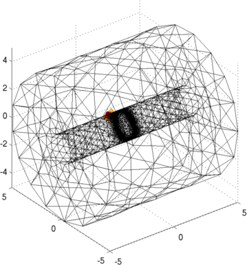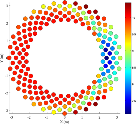
Figure: Forward model including a cavity and pseudo-section for circumferential outward measurements using a Wenner protocol.

Case of circumferential measurements around a cylinder

% Forward Model of a cylindrical object
% Create 3D model of a tunnel $Id: stimPatt_PseudoSec08.m 3902 2013-04-18 17:59:23Z aadler $
n_elec = 32;
shape_str = ['solid incyl  = cylinder (0,0,0; 1,0,0; 1) -maxh=1.0; \n', ...
    'solid pl1    =  plane(-.5,0,0;-1,0,0);\n' ...
    'solid pl2    =  plane( .5,0,0; 1,0,0);\n' ...
    'solid mainobj= pl1 and pl2 and incyl;\n'];
th= linspace(0,2*pi,n_elec+1)'; th(end)=[];
cth= cos(th); sth=sin(th); zth= zeros(size(th));
elec_pos = [zth, cth, sth, zth cth, sth];
elec_shape= 0.01;
elec_obj = 'incyl';
fmdl = ng_mk_gen_models(shape_str, elec_pos, elec_shape, elec_obj);


% Construct the Wenner stimulation pattern
 fmdl.stimulation= stim_pattern_geophys( n_elec, 'Wenner', {'spacings',1:6,'circumferential_meas',1} );
%fmdl.stimulation= mk_stim_patterns(n_elec, 1, [0,3],[0,3],{},1);

% Use apparent_resistivity
fmdl.jacobian = @jacobian_apparent_resistivity;
fmdl.solve    = @fwd_solve_apparent_resistivity;

% Construct a model with a homogeneous conductivity of 0.1 Sm and insert a conductive sphere
img = mk_image(fmdl,0.1+ mk_c2f_circ_mapping(fmdl,[0;0.8;0;0.1])*100);
show_fem(img);
print_convert stimPatt_PseudoSec08_1.png '-density 75'

% Solve the forward problem
dd  = fwd_solve(img);

% Show the pseudo-section of the apparent resistivity
fmdl.show_pseudosection.orientation = {'CircularInside','yz'};
show_pseudosection( fmdl, dd.meas);

print_convert stimPatt_PseudoSec08_2.png '-density 75'

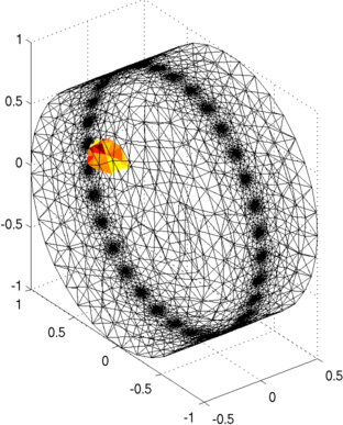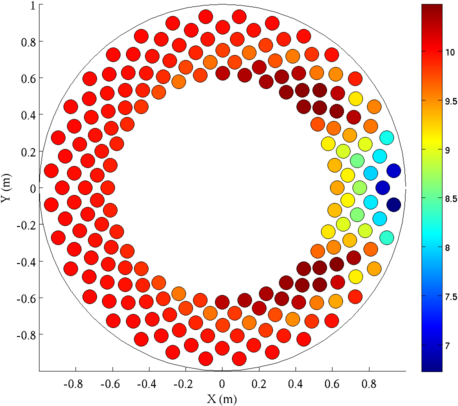
Figure: Forward model around a cylinder and pseudo-section for circumferential inward measurements using a Wenner protocol.