EIDORS: Electrical Impedance Tomography and Diffuse Optical Tomography Reconstruction Software

Hosted by

Images of the Pont Péan region

The data are available here. They were measured by a team of geophysical researchers at Université Rennes 1 over the period 2000−2011.

Create 3D FEM model of the terrain

% Load data and positions
gps = load('Mine_20FEV2004.gps');
data= load('Mine_20FEV2004_LI.tomel');

% Forward Model
shape_str = ['solid top    = plane(0,0,0;0,1,0);\n' ...
             'solid mainobj= top and orthobrick(-100,-200,-100;425,10,100) -maxh=20.0;\n'];
elec_pos = gps(:,2:4); e0 = elec_pos(:,1)*0;
elec_pos = [  elec_pos, e0, e0+1, e0 ]; 
elec_shape=[0.5,.5,.5];
elec_obj = 'top';
fmdl = ng_mk_gen_models(shape_str, elec_pos, elec_shape, elec_obj);

fmdl.stimulation = stim_meas_list( data(:,3:6) - 40100);

show_fem(fmdl);

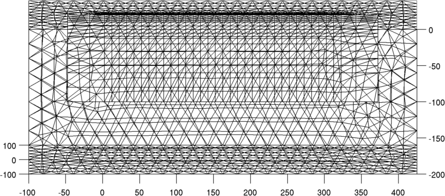
Figure: Forward model

Create 2½D inverse model

%Reconstruction model
[cmdl]= mk_grid_model([], 2.5+[-50,-20,0:10:320,340,370], ...
                             -[0:2.5:10, 15:5:25,30:10:80,100,120]);
c2f = mk_coarse_fine_mapping( fmdl, cmdl);

fmdl.coarse2fine = c2f;
imdl= eidors_obj('inv_model','test');
imdl.fwd_model= fmdl;
imdl.rec_model= cmdl;
   imdl.reconst_type = 'difference';
   imdl.RtR_prior = @prior_laplace;
   imdl.solve = @inv_solve_diff_GN_one_step;
   imdl.hyperparameter.value = 0.3;
   imdl.fwd_model.normalize_measurements = 1;
   imdl.jacobian_bkgnd.value = 0.03;

hold on
show_fem(cmdl);
view([0 -0.2 1])
hold off
print_convert pont_pean01a.png

Reconstruct the data

% Difference image vs simulated data
vr = data(:,9);
img = mk_image( imdl );
vh = fwd_solve(img); vh = vh.meas;

imgr = inv_solve(imdl, vh, vr);

show_fem(imgr);
print_convert pont_pean3a.png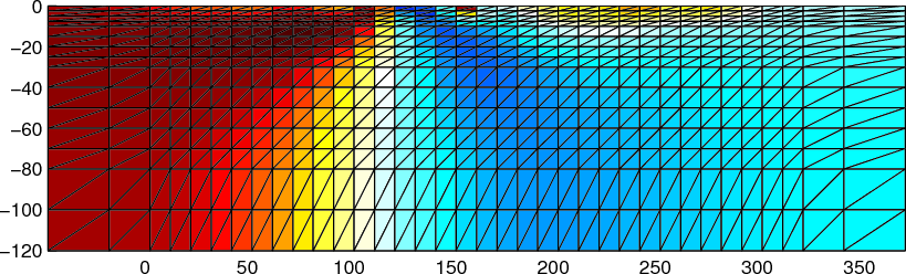

Figure: Reconstruction (2½D) using a one step GN algorithm

Comparison to Apparent Resistivity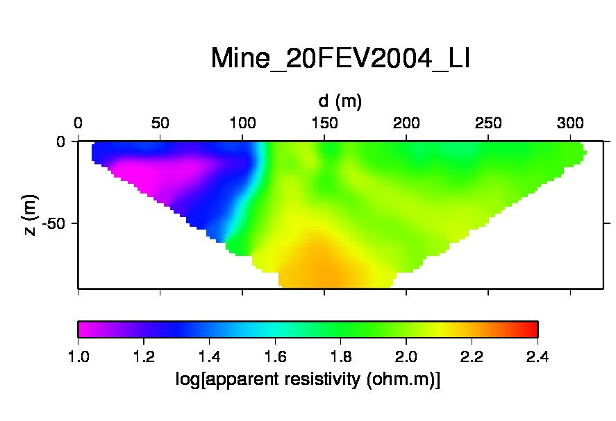

Figure: Apparent resistivity plot (not using EIDORS)