|
|
EIDORS: Electrical Impedance Tomography and Diffuse Optical Tomography Reconstruction Software |
|
EIDORS
(mirror) Main Documentation Tutorials − Image Reconst − Data Structures − Applications − FEM Modelling − GREIT − Old tutorials − Workshop Download Contrib Data GREIT Browse Docs Browse SVN News Mailing list (archive) FAQ Developer
Hosted by |
Two and a half dim (2½D) image reconstructionThe term "2½D" or 2.5D originates from geophysics. Measurements are made around a medium (or in a borehole) in 3D. However, in order to simplify image reconstruction, the medium properties are assumed to be constant in the z direction.Thus, the z direction is part of the forward model, but not the inverse. It is thus "half" a dimension. Fourier ApproximationThe 2½D is typically built by constructing a 2D forward model and approximating the effect of the additional z direction through a summation of Fourier transform coefficients. Depending on the formulation, the Fourier summation may represent a finite region on either (for example, a cylinder) or an infinitely large region (for example, a half-space). Course/fine mapping can be applied on top of this to give a fine 2D forward model and a coarse 2D inverse model. The electrodes must all be at the z=0 plane.
For an explanation of the formulation, see the presentation for
Generally, the formulation used in geophysics uses Point Electrodes Models (PEM). Here we use the Complete Electrode Model (CEM) in the x and y directions, and the PEM in the z direction.
% Models
fmdl = mk_common_model('d2C',16); % fine model
cmdl = mk_common_model('c2C',16); % coarse model
c2f = mk_coarse_fine_mapping(fmdl.fwd_model, cmdl.fwd_model);
imdl = fmdl;
imdl.rec_model = cmdl.fwd_model;
imdl.fwd_model.coarse2fine = c2f;

clf; % figure 1
subplot(121);show_fem(imdl.fwd_model);
title('fine (2d) model'); axis square; axis off;
subplot(122); show_fem(imdl.rec_model);
title('coarse (2d) model'); axis square; axis off;
print_convert two_and_half_d01a.png '-density 75'
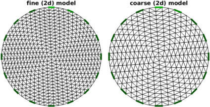
Figure: Left fine (2d) model, Right coarse (2d) model
% test c2f
rimg = mk_image(cmdl,1);
rimg.fwd_model = imdl.fwd_model;
rimg.rec_model = imdl.rec_model;
rimg.elem_data = 1 + ...
   elem_select( rimg.rec_model, '(x-0.3).^2+(y+0.1).^2<0.15^2' ) - ...
   elem_select( rimg.rec_model, '(x+0.4).^2+(y-0.2).^2<0.2^2' )*0.5;
fimg = mk_image(fmdl,1);
fimg.elem_data = 1 + ...
   elem_select( rimg.fwd_model, '(x-0.3).^2+(y+0.1).^2<0.15^2' ) - ...
   elem_select( rimg.fwd_model, '(x+0.4).^2+(y-0.2).^2<0.2^2' )*0.5;
clf; % figure 1
subplot(131); show_fem(mk_image(imdl.rec_model,rimg.elem_data)); axis square; axis off;
title('coarse');
subplot(132); show_fem(mk_image(imdl.fwd_model,c2f*rimg.elem_data)); axis square; axis off;
title('coarse-to-fine');
subplot(133); show_fem(fimg); axis square; axis off; title('fwd fine');
print_convert two_and_half_d02a.png '-density 75';

% Simulate data - homogeneous
himg = mk_image(fmdl,1);
vh = fwd_solve_2p5d_1st_order(himg);
% Simulate data - inhomogeneous
vi = fwd_solve_2p5d_1st_order(fimg);
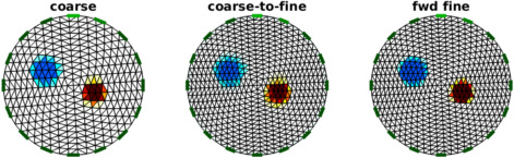
Figure: Left coarse model Centre coarse data mapped to fine model Right fine model
% Solve 2.5D
% Create inverse Model: Classic
imdl.hyperparameter.value = .1;
imdl.reconst_type = 'difference';
imdl.type = 'inv_model';

% Classic and 2.5D (inverse crime) solver
vh.type = 'data';
vi.type = 'data';
img2 = inv_solve(imdl, vh, vi);
imdl.fwd_model.jacobian = @jacobian_adjoint_2p5d_1st_order;
img25 = inv_solve(imdl, vh, vi);

clf;
subplot(131); show_fem(fimg); title('model'); axis off; axis square;
subplot(132); show_fem(img2); title('2D'); axis off; axis square;
subplot(133); show_fem(img25);title('2.5D'); axis off; axis square;
print_convert two_and_half_d03a.png
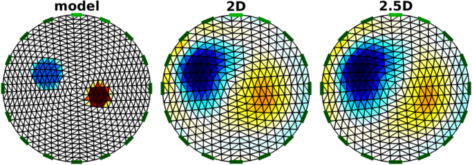
Figure: Left original model Centre 2d reconstruction Right 2½ reconstruction onto coarse model 2D + 3D = 2.5DThe 2½D can also be built as an application of coarse/fine mapping, where the fine (high density) 3D forward model is used with a coarse (low density) 2D inverse model. The 2D model is projected through the 3D model giving constant conductivity along the axis of the projection.
% Build 2D and 3D model $Id: two_and_half_d04.m 5392 2017-04-12 05:22:03Z alistair_boyle $

demo_img = mk_common_model('n3r2',[16,2]);

% Create 2D FEM of all NODES with z=0
f_mdl = demo_img.fwd_model;
n2d = f_mdl.nodes( (f_mdl.nodes(:,3) == 0), 1:2);
e2d = delaunayn(n2d);
c_mdl = eidors_obj('fwd_model','2d','elems',e2d,'nodes',n2d);

subplot(121);
show_fem(f_mdl); title('fine (3d) model');

subplot(122);
show_fem(c_mdl); title('coarse (2d) model');
axis square

print_convert two_and_half_d04a.png '-density 75'

% Simulate data - inhomogeneous
img = mk_image(demo_img,1);
vi= fwd_solve(img);

% Simulate data - homogeneous
load( 'datacom.mat' ,'A','B')
img.elem_data(A)= 1.15;
img.elem_data(B)= 0.80;
vh= fwd_solve(img);
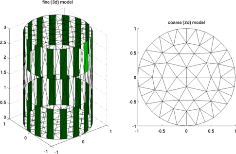
Figure: Left fine (3d) model, Right coarse (2d) model
% Solve 2D and 3D model $Id: two_and_half_d05.m 5392 2017-04-12 05:22:03Z alistair_boyle $

% Original target
subplot(141)
show_fem(img); view(-62,28)

% Create inverse Model: Classic
imdl= select_imdl(f_mdl, {'Basic GN dif'});
imdl.hyperparameter.value = .1;

% Classic (inverse crime) solver
img1= inv_solve(imdl, vh, vi);
subplot(142)
show_fem(img1); view(-62,28)
Next, create geometries for the fine and
coarse mesh.
Images are reconstructed by calling the
coase_fine_solver function rather
than the original. (Note this function
still needs some work, it doesn't account for
all cases)
% Solve 2D and 3D model $Id: two_and_half_d06.m 5392 2017-04-12 05:22:03Z alistair_boyle $

c2f= mk_coarse_fine_mapping( f_mdl, c_mdl );

imdl.fwd_model.coarse2fine = c2f;
img2= inv_solve(imdl, vh, vi);
img2.elem_data= c2f*img2.elem_data;
subplot(143)
show_fem(img2); view(-62,28)

% 2.5D reconstruct onto coarse model
subplot(144)
img3= inv_solve(imdl, vh, vi);
img3.fwd_model= c_mdl;
show_fem(img3);
zlim([0,3]); xlim([-1,1]); ylim([-1,1]);
 axis equal; view(-62,28)

print_convert two_and_half_d06a.png
Note the reconstructed image on the coarse mesh is extruded into 2D, as the assumptions require. 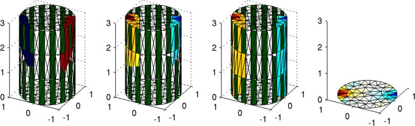
Figure: Left original (3d) model Centre left fine (3d) reconstruction Centre right 2½ reconstruction onto fine model Right 2½ reconstruction onto coarse model |
Last Modified: $Date: 2017-04-12 01:30:57 -0400 (Wed, 12 Apr 2017) $ by $Author: alistair_boyle $