EIDORS: Electrical Impedance Tomography and Diffuse Optical Tomography Reconstruction Software

Hosted by

Model of a 2½D cross-section of a pipe

Using netgen, we simulate a cylindrical pipe with one row of 12 electrodes.

% Create pipe model $Id: pipe01.m 2195 2010-06-19 08:49:47Z aadler $

n_elec = 12;
stim= mk_stim_patterns( n_elec, 1, [0,3],[0,1],{},1);

fmdl= ng_mk_cyl_models(4,[n_elec,2],[0.2,0.5,0.04]);
fmdl.stimulation = stim;

clf; subplot(121);
show_fem(fmdl)
print_convert('pipe01a.png','-density 100')

show_fem(fmdl); view([0,0]);
print_convert('pipe01b.png','-density 90')

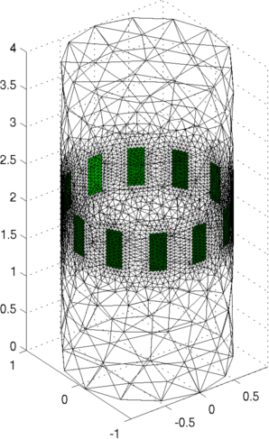
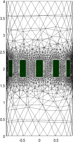
Figure: Netgen model of a pipe with a row of electrodes around the centre from two view points.

Simulate an elliptical fluid moves in the pipe

% Create pipe model $Id: pipe02.m 3266 2012-06-30 16:01:06Z aadler $

el= 'ellipsoid(0.3,0.2,1.5; 0,0,0.25; 0.1,0,0; 0,0.1,0)';
extra={'obj',['solid obj = ',el,';']};

fmdl= ng_mk_cyl_models(4,[n_elec,2],[0.2,0.5,0.04], extra);
fmdl.stimulation = stim;

img= mk_image(fmdl, 1);
vh = fwd_solve( img );
img.elem_data(fmdl.mat_idx{2}) = 2;
vi = fwd_solve( img );

clf; subplot(121);
show_fem(img); view([0,0]);
print_convert('pipe02a.png','-density 100')

clf; plot( [vh.meas, 100*(vi.meas - vh.meas)] )
print_convert('pipe02b.png','-density 75')

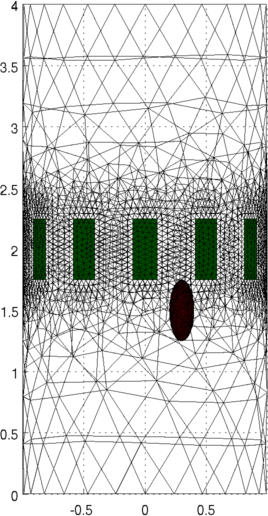
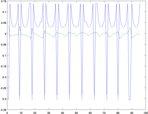
Figure: Left: elliptic conductive object in pipe Right: homogeneous and difference voltages due to object

Create reconstruction model

First, we create a coarse model which represents the entire depth in z (ie. like the 2½D model).

% Create coarse model
imdl= mk_common_model('b2c2',16);
cmdl= imdl.fwd_model;

scl = 1;
cmdl.mk_coarse_fine_mapping.f2c_offset = [0,0,1];
cmdl.mk_coarse_fine_mapping.f2c_project = (1/scl)*speye(3);
cmdl.mk_coarse_fine_mapping.z_depth = inf;
c2f= mk_coarse_fine_mapping( fmdl, cmdl);

% Create reconstruction model
imdl.rec_model= cmdl;
imdl.fwd_model= fmdl;
imdl.fwd_model.coarse2fine = c2f;
imdl.RtR_prior = @prior_gaussian_HPF;
imdl.solve = @inv_solve_diff_GN_one_step;
imdl.hyperparameter.value= .01;

imgc= inv_solve(imdl, vh, vi);

show_fem(imgc);
print_convert pipe03a.png '-density 75';

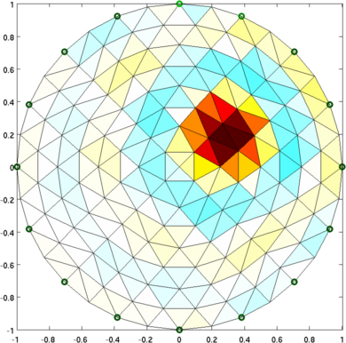
Figure:

cmdl.mk_coarse_fine_mapping.z_depth = 0.1;
c2f= mk_coarse_fine_mapping( fmdl, cmdl);

% modify
imdl.fwd_model.coarse2fine = c2f;
imdl.hyperparameter.value = .01;

imgc= inv_solve(imdl, vh, vi);
imgc.calc_colours.ref_level= 0;

show_fem(imgc);
print_convert pipe04a.png '-density 75';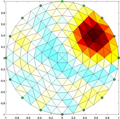

Figure: