EIDORS: Electrical Impedance Tomography and Diffuse Optical Tomography Reconstruction Software

Hosted by

Dual Models to reconstruct a slice of a volume

To simulate this, we simulate a ball moving in a helical path on a fine netgen model.

% Simulate Moving Ball - Helix $Id: centre_slice01.m 2666 2011-07-12 20:41:02Z aadler $

% get ng_mdl_16x2_vfine from data_contrib section of web page
n_sims= 20;
stim = mk_stim_patterns(16,2,'{ad}','{ad}',{},1);
fmdl = mk_library_model('cylinder_16x2el_vfine');
fmdl.stimulation = stim;
[vh,vi,xyzr_pt]= simulate_3d_movement( n_sims, fmdl);

clf; show_fem(fmdl)
crop_model(gca, inline('x-z<-15','x','y','z'))
view(-23,14)

hold on
[xs,ys,zs]=sphere(10);
for i=1:n_sims
   xp=xyzr_pt(1,i); yp=xyzr_pt(2,i);
   zp=xyzr_pt(3,i); rp=xyzr_pt(4,i);
   hh=surf(rp*xs+xp, rp*ys+yp, rp*zs+zp);
   set(hh,'EdgeColor',[.4,0,.4],'FaceColor',[.2,0,.2]);
end
hold off

print_convert centre_slice01a.png '-density 100'

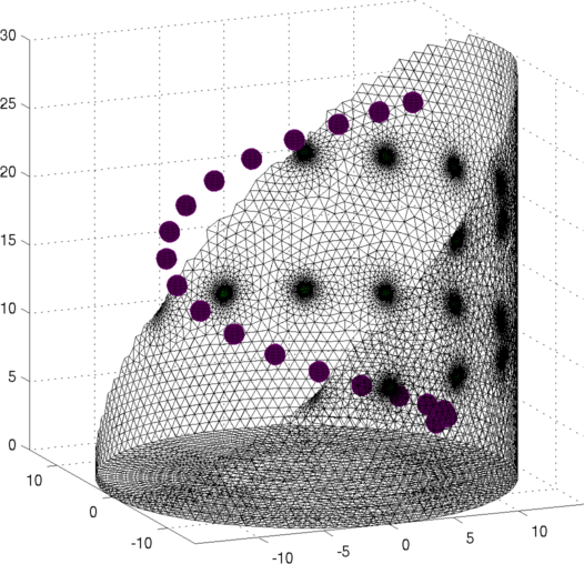
Figure: Netgen model of a 2×16 electrode tank. The positions of the simulated conductive target moving in a helical path are shown in purple.

Create reconstruction model

% 2D solver $Id: centre_slice02.m 2666 2011-07-12 20:41:02Z aadler $

% Create and show inverse solver
imdl = mk_common_model('b3cr',[16,2]);

f_mdl = mk_library_model('cylinder_16x2el_coarse');
f_mdl.stimulation = stim;
imdl.fwd_model = f_mdl;

% Create coarse model
imdl2d= mk_common_model('b2c2',16);
c_mdl= imdl2d.fwd_model;

% Show fine model
show_fem(f_mdl);
crop_model(gca, inline('x-z<-15','x','y','z'))
view(-23,10)

scl= 15; % scale difference between c_mdl and f_mdl
c_els= c_mdl.elems;
c_ndsx= c_mdl.nodes(:,1)*scl;
c_ndsy= c_mdl.nodes(:,2)*scl;
c_ndsz= 0*c_ndsx; 

layersep= .3;
layerhig= .1;
hold on
% Lower resonstruction layer
hh= trimesh(c_els, c_ndsx, c_ndsy, c_ndsz+(1-layersep)*scl);
set(hh, 'EdgeColor', [1,0,0]);
hh= trimesh(c_els, c_ndsx, c_ndsy, c_ndsz+(1-layersep-layerhig)*scl);
set(hh, 'EdgeColor', [.3,.3,.3]);
hh= trimesh(c_els, c_ndsx, c_ndsy, c_ndsz+(1-layersep+layerhig)*scl);
set(hh, 'EdgeColor', [.3,.3,.3]);

% Upper resonstruction layer
hh= trimesh(c_els, c_ndsx, c_ndsy, c_ndsz+(1+layersep)*scl);
set(hh, 'EdgeColor', [0,0,1]);
hh= trimesh(c_els, c_ndsx, c_ndsy, c_ndsz+(1+layersep-layerhig)*scl);
set(hh, 'EdgeColor', [.3,.3,.3]);
hh= trimesh(c_els, c_ndsx, c_ndsy, c_ndsz+(1+layersep+layerhig)*scl);
set(hh, 'EdgeColor', [.3,.3,.3]);

for i=1:n_sims
   xp=xyzr_pt(1,i); yp=xyzr_pt(2,i);
   zp=xyzr_pt(3,i); rp=xyzr_pt(4,i);
   hh=surf(rp*xs+xp, rp*ys+yp, rp*zs+zp);
   set(hh,'EdgeColor',[.4,0,.4]);
end

hold off;

print_convert centre_slice02a.png '-density 100'

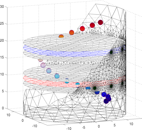
Figure: Netgen model of a 2×16 electrode tank. The positions of the simulated conductive target moving in a helical path are shown in purple. The 3D fine model is shown (cropped). The upper (blue) and lower (red) layers corresponding to the geometry of the coarse model are shown. The z direction limits of the coarse model are shown in grey.

Image reconstructions

% 2D solver $Id: centre_slice03.m 4839 2015-03-30 07:44:50Z aadler $


% Set coarse as reconstruction model
imdl.rec_model= c_mdl;
c_mdl.mk_coarse_fine_mapping.f2c_offset = [0,0,scl];
c_mdl.mk_coarse_fine_mapping.f2c_project = (1/scl)*speye(3);
c_mdl.mk_coarse_fine_mapping.z_depth = inf;
c2f= mk_coarse_fine_mapping( f_mdl, c_mdl);
imdl.fwd_model.coarse2fine = c2f;
imdl.RtR_prior = @prior_gaussian_HPF;
imdl.solve = @inv_solve_diff_GN_one_step;
imdl.hyperparameter.value= 0.1;

imgc= inv_solve(imdl, vh, vi);

clf; show_slices(imgc);
print_convert centre_slice04a.png '-density 75';

% 2D solver $Id: centre_slice04.m 4839 2015-03-30 07:44:50Z aadler $

imdl.hyperparameter.value= 0.05;

c_mdl.mk_coarse_fine_mapping.f2c_offset = [0,0,(1-.3)*scl];
c_mdl.mk_coarse_fine_mapping.z_depth = 0.1;
c2f= mk_coarse_fine_mapping( f_mdl, c_mdl);
imdl.fwd_model.coarse2fine = c2f;
imgc0= inv_solve(imdl, vh, vi);
% Show image of reconstruction in upper planes
show_slices(imgc0);
print_convert centre_slice04b.png '-density 75';

c_mdl.mk_coarse_fine_mapping.f2c_offset = [0,0,(1+.3)*scl];
c_mdl.mk_coarse_fine_mapping.z_depth = 0.1;
c2f= mk_coarse_fine_mapping( f_mdl, c_mdl);
imdl.fwd_model.coarse2fine = c2f;
imgc1= inv_solve(imdl, vh, vi);

% Show image of reconstruction in lower planes
show_slices(imgc1);
print_convert centre_slice04c.png '-density 75';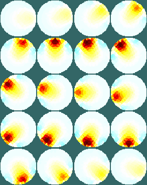

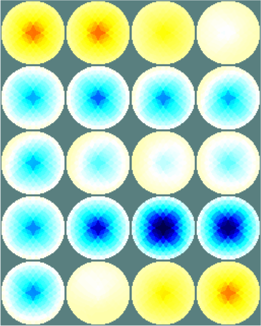
Figure: Reconstructed images of a target moving in a helical pattern using difference coarse models Left coarse model with z_depth=∞ Centrecoarse model with z_depth=0.1×scale at upper position Right coarse model with z_depth=0.1×scale at lower positions

Simpler reconstruction model

% 2D solver $Id: centre_slice05.m 2673 2011-07-13 06:57:41Z aadler $

% Create and show inverse solver
imdl = mk_common_model('b3cr',[16,2]);
f_mdl= imdl.fwd_model;

% Create coarse model
imdl2d= mk_common_model('b2c2',16);
c_mdl= imdl2d.fwd_model;

% Show fine model
clf;show_fem(f_mdl);
crop_model(gca, inline('x-z<-.5','x','y','z'))
view(-23,10)

scl= 1; % scale difference between c_mdl and f_mdl
c_els= c_mdl.elems;
c_ndsx= c_mdl.nodes(:,1)*scl;
c_ndsy= c_mdl.nodes(:,2)*scl;
c_ndsz= 0*c_ndsx; 

layersep= .3;
layerhig= .1;
hold on
% Lower resonstruction layer
hh= trimesh(c_els, c_ndsx, c_ndsy, c_ndsz+(-layersep)*scl);
set(hh, 'EdgeColor', [1,0,0]);
hh= trimesh(c_els, c_ndsx, c_ndsy, c_ndsz+(-layersep-layerhig)*scl);
set(hh, 'EdgeColor', [.3,.3,.3]);
hh= trimesh(c_els, c_ndsx, c_ndsy, c_ndsz+(-layersep+layerhig)*scl);
set(hh, 'EdgeColor', [.3,.3,.3]);

% Upper resonstruction layer
hh= trimesh(c_els, c_ndsx, c_ndsy, c_ndsz+(+layersep)*scl);
set(hh, 'EdgeColor', [0,0,1]);
hh= trimesh(c_els, c_ndsx, c_ndsy, c_ndsz+(+layersep-layerhig)*scl);
set(hh, 'EdgeColor', [.3,.3,.3]);
hh= trimesh(c_els, c_ndsx, c_ndsy, c_ndsz+(+layersep+layerhig)*scl);
set(hh, 'EdgeColor', [.3,.3,.3]);

[xs,ys,zs]=sphere(10);
for i=1:size(xyzr_pt,2)
   xp=xyzr_pt(1,i)/15;   yp=xyzr_pt(2,i)/15;
   zp=xyzr_pt(3,i)/15-1; rp=xyzr_pt(4,i)/15;
   hh=surf(rp*xs+xp, rp*ys+yp, rp*zs+zp);
   set(hh,'EdgeColor',[.4,0,.4]);
end

hold off;

print_convert centre_slice05a.png '-density 100';

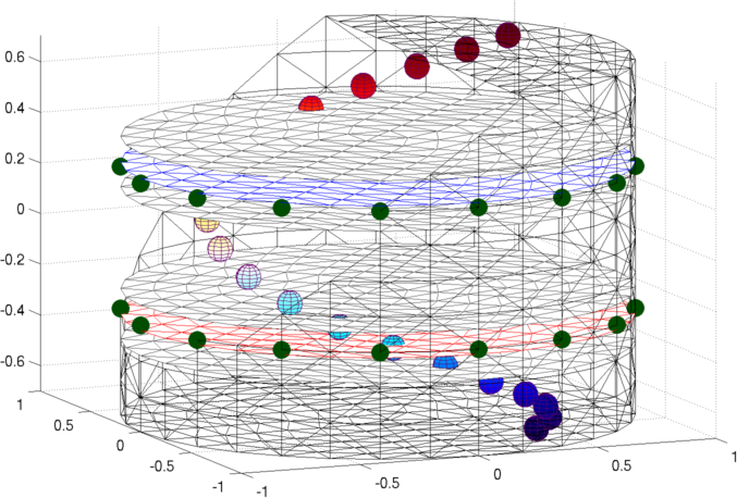
Figure: Simple extruded model of a 2×16 electrode tank. The positions of the simulated conductive target moving in a helical path are shown in purple. The 3D fine model is shown (cropped). The upper (blue) and lower (red) layers corresponding to the geometry of the coarse model are shown. The z direction limits of the coarse model are shown in grey.

Image reconstructions

% 2D solver $Id: centre_slice06.m 4839 2015-03-30 07:44:50Z aadler $

% Set coarse as reconstruction model
imdl.rec_model= c_mdl;
c2f= mk_coarse_fine_mapping( f_mdl, c_mdl);
imdl.fwd_model.coarse2fine = c2f;
imdl.RtR_prior = @prior_gaussian_HPF;
imdl.solve = @inv_solve_diff_GN_one_step;
imdl.hyperparameter.value= 0.2;

imgc= inv_solve(imdl, vh, vi);
clf; show_slices(imgc);
print_convert centre_slice06a.png '-density 75';

c_mdl.mk_coarse_fine_mapping.f2c_offset = [0,0,-.3];
c_mdl.mk_coarse_fine_mapping.z_depth = 0.1;
c2f= mk_coarse_fine_mapping( f_mdl, c_mdl);
imdl.fwd_model.coarse2fine = c2f;
imgc0= inv_solve(imdl, vh, vi);

imgc0= inv_solve(imdl, vh, vi);
show_slices(imgc0);
print_convert centre_slice06b.png '-density 75';

c_mdl.mk_coarse_fine_mapping.f2c_offset = [0,0,.3];
c_mdl.mk_coarse_fine_mapping.z_depth = 0.1;
c2f= mk_coarse_fine_mapping( f_mdl, c_mdl);
imdl.fwd_model.coarse2fine = c2f;

imgc1= inv_solve(imdl, vh, vi);
show_slices(imgc1);
print_convert centre_slice06c.png '-density 75';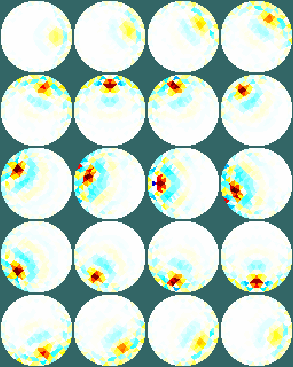

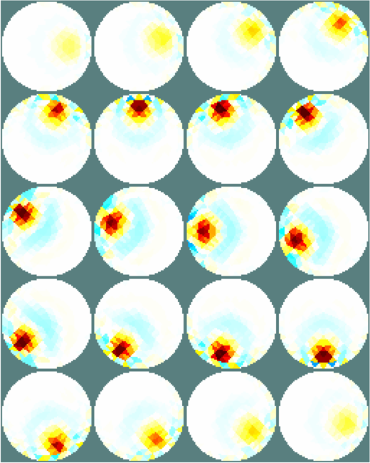
Figure: Reconstructed images of a target moving in a helical pattern using difference coarse models Left coarse model with z_depth=∞ Centrecoarse model with z_depth=0.1×scale at upper position Right coarse model with z_depth=0.1×scale at lower positions