EIDORS: Electrical Impedance Tomography and Diffuse Optical Tomography Reconstruction Software

Hosted by

Simulate a moving 2D target on a fixed mesh

Step 1: Create fine mesh (300 nodes)

% create model $Id: simulate_move2_01.m 2796 2011-07-14 23:14:21Z bgrychtol $

% Model parameters
n_elec= 16;
n_nodes= 300;

% Create electrodes
refine_level=4; %electrode refinement level
elec_width= .1;
z_contact = 0.01;
% elect positions
th=linspace(0,2*pi,n_elec(1)+1)';th(end)=[];
elec_posn= [sin(th),cos(th)];
[elec_nodes, refine_nodes] = dm_mk_elec_nodes( elec_posn, ...
       elec_width, refine_level);

% Define circular medium
fd=inline('sum(p.^2,2)-1','p');
bbox = [-1,-1;1,1];
smdl= dm_mk_fwd_model( fd, [], n_nodes, bbox, ...
                          elec_nodes, refine_nodes, z_contact);

Step 2: Simulate movement

% create model $Id: simulate_move2_02.m 2781 2011-07-14 21:06:54Z bgrychtol $

% Create an object within the model
trg_ctr= [.7,.1];
trg_rad= 0.1;
th=linspace(0,2*pi,20)';th(end)=[];
trg_refine_nodes= [refine_nodes; ...
             trg_rad*sin(th)+trg_ctr(1), ...
             trg_rad*cos(th)+trg_ctr(2) ];

tmdl= dm_mk_fwd_model( fd, [], n_nodes, bbox, elec_nodes, ...
                       trg_refine_nodes, z_contact);

% find elements in size target
mdl_pts = interp_mesh( tmdl );
ctr_pts = mdl_pts - ones(size(mdl_pts,1),1)*trg_ctr;
in_trg  =(sum(ctr_pts.^2,2) < trg_rad^2);


timg= eidors_obj('image','','fwd_model',tmdl,...
                 'elem_data',1 + in_trg*.5);

% Show output - full size
subplot(121); show_fem( smdl ); axis equal; axis([-1.1 1.1 -1.1 1.1]);  
subplot(122); show_fem( timg ); axis equal; axis([-1.1 1.1 -1.1 1.1]);
print_convert simulate_move2_02a.png '-density 125'

% Show output - full size
subplot(121); show_fem( smdl ); axis equal; axis([.5,1.05,-.1,.3]);
subplot(122); show_fem( timg ); axis equal; axis([.5,1.05,-.1,.3]); 
print_convert simulate_move2_02b.png '-density 125'

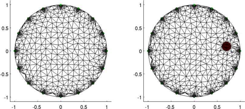
Figure: Left Simulation mesh homogeneous mesh Right Simulation mesh with target at (0.1,0.7)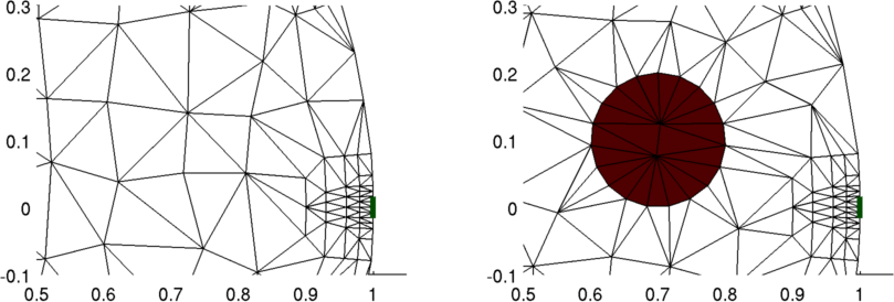

Figure: Magnification of areas of interest in the previous figure. Left Simulation mesh homogeneous mesh Right Simulation mesh with target at (0.1,0.7)

Step 3: Simulate Homogeneous measurements

% simulate homogeneous $Id: simulate_move2_03.m 3273 2012-06-30 18:00:35Z aadler $

% stimulation pattern: adjacent
stim_pat= mk_stim_patterns(n_elec,1,'{ad}','{ad}',{},1);

smdl.stimulation= stim_pat;
himg= mk_image(smdl, 1);

vh= fwd_solve(himg);

Step 4: Simulate moving target and simulate measurements

% moving target $Id: simulate_move2_04.m 3273 2012-06-30 18:00:35Z aadler $

% Create a moving object within the model
trg_rad= 0.1;
radius= 0.75;
n_sims= 20;
contrast= 0.1;

clear vi;
for i= 1:n_sims;
   thc= 2*pi*(i-1)/n_sims;
   trg_ctr= radius*[cos(thc),sin(thc)];

   trg_refine_nodes= [refine_nodes; ...
                trg_rad*sin(th)+trg_ctr(1), ...
                trg_rad*cos(th)+trg_ctr(2) ];

   tmdl= dm_mk_fwd_model( fd, [], n_nodes, bbox, elec_nodes, ...
                          trg_refine_nodes, z_contact);
   tmdl.stimulation = stim_pat;

   % find elements in size target
   mdl_pts = interp_mesh( tmdl );
   ctr_pts = mdl_pts - ones(size(mdl_pts,1),1)*trg_ctr;
   in_trg  =(sum(ctr_pts.^2,2) < trg_rad^2);

   % Create target image object
   timg= mk_image(tmdl,1 + in_trg*contrast);

   clf; show_fem(timg); axis equal
   print_convert(sprintf('simulate_move2_04a%02d.png',i),'-density 50');
   vi(i)= fwd_solve(timg);
end

% Create animated graphics $Id: simulate_move2_05.m 1535 2008-07-26 15:36:27Z aadler $

% Trim images
!find -name 'simulate_move2_04a*.png' -exec convert  -trim '{}' PNG8:'{}' ';'

% Convert to animated Gif
!convert -delay 50 simulate_move2_04a*.png -loop 0 simulate_move2_05a.gif

Figure: Animation of the simulation mesh surrounding a moving target

Step 5: Reconstruct images

% Reconstruct images $Id: simulate_move2_06.m 2781 2011-07-14 21:06:54Z bgrychtol $

imdl= mk_common_model('c2c2',16);
img= inv_solve(imdl, vh, vi);
subplot(121); show_fem(img); axis image
subplot(122); show_slices(img)

print_convert simulate_move2_06a.png '-density 125'

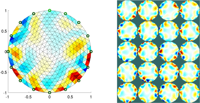
Figure: Reconstructed images of targets moving in the mesh Left Reconstruction mesh with first image Right Reconstructed images of all targets

Exploring the effect of mesh density

Mesh with n_nodes=500 and refine_level=2

Figure: Animation of the simulation mesh surrounding a moving target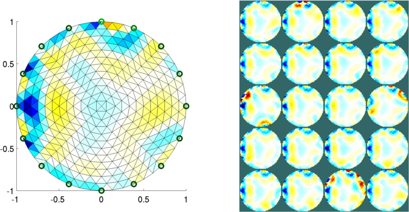

Figure: Reconstructed images of targets moving in the mesh Left Reconstruction mesh with first image Right Reconstructed images of all targets

Mesh with n_nodes=1000 and refine_level=4

Figure: Animation of the simulation mesh surrounding a moving target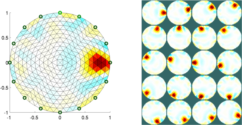

Figure: Reconstructed images of targets moving in the mesh Left Reconstruction mesh with first image Right Reconstructed images of all targets