EIDORS: Electrical Impedance Tomography and Diffuse Optical Tomography Reconstruction Software

Hosted by

Noise performance of different hyperparameter selection approaches

1. NF - noise figure as suggested by Adler et al. (1996)
2. SNR - image SNR as suggested by Braun et al. (2017)
3. LCV - L-curve criterion as suggested by Hansen et al. (1993)
4. GCV - generalized cross-validation as suggested by Golub et al. (1979)

Fabian Braun, Martin Proença, Josep Solà, Jean-Philippe Thiran and Andy Adler A Versatile Noise Performance Metric for Electrical Impedance Tomography Algorithms IEEE Transactions on Biomedical Engineering, 64(10):2321-2330, 2017, DOI: 10.1109/TBME.2017.2659540.

Human thorax model with different electrode configurations

1. 16 elecs, skip 0: 16 equidistantly spaced electrodes, and skip 0 (adjacent) stim/meas pattern
2. 16 elecs, skip 5: 16 equidistantly spaced electrodes, and skip 5 stim/meas pattern
3. 32 elecs, skip 0: 32 equidistantly spaced electrodes, and skip 0 (adjacent) stim/meas pattern
4. 24 elecs, skip 9: 24 electrodes spaced more densely ventrally, and skip 9 stim/meas pattern

% create forward models of the human thorax 
% $Id: noise_performance_01.m 5424 2017-04-25 17:45:19Z aadler $

% generate base model for forward solving
fmdl = mk_library_model('adult_male_32el_lungs');
imgBasic = mk_image(fmdl, 0.2);     % back ground conductivity
imgBasic.elem_data(fmdl.mat_idx{2}) = 0.13;   % left lung
imgBasic.elem_data(fmdl.mat_idx{3}) = 0.13;   % right lung
imgBasic.elem_data1 = imgBasic.elem_data;
% now generate a conductivity change
imgBasic.elem_data2 = imgBasic.elem_data;
imgBasic.elem_data2(fmdl.mat_idx{2}) = 0.1 * imgBasic.elem_data2(fmdl.mat_idx{2});
imgBasic.elem_data2(fmdl.mat_idx{3}) = 0.05 * imgBasic.elem_data2(fmdl.mat_idx{3}); 

% generate base model for inverse model
rmdlBasic = mk_library_model('adult_male_32el');

% 16 electrodes, equidistantly spaced, skip 0 (adjacent) stim/meas pattern
imgs{1} = imgBasic;
rmdls{1} = rmdlBasic;
imgs{1}.fwd_model.electrode(2:2:end) = []; 
imgs{1}.fwd_model.name = '16 elecs, skip 0';
rmdls{1}.electrode(2:2:end) = [];
imgs{1}.fwd_model.stimulation = mk_stim_patterns(16,1,[0,1],[0,1],{'no_rotate_meas','no_meas_current'});
rmdls{1}.stimulation = imgs{1}.fwd_model.stimulation;

% 16 electrodes, equidistantly spaced, stim/meas pattern with skip=5
imgs{2} = imgBasic;
rmdls{2} = rmdlBasic;
imgs{2}.fwd_model.electrode(2:2:end) = []; 
imgs{2}.fwd_model.name = '16 elecs, skip 5';
rmdls{2}.electrode(2:2:end) = [];
imgs{2}.fwd_model.stimulation = mk_stim_patterns(16,1,[0,1+5],[0,1+5],{'no_rotate_meas','no_meas_current'});
rmdls{2}.stimulation = imgs{2}.fwd_model.stimulation;

% 32 electrodes, equidistantly spaced, skip 0 (adjacent) stim/meas pattern
imgs{3} = imgBasic;
rmdls{3} = rmdlBasic;
imgs{3}.fwd_model.name = '32 elecs, skip 0';
imgs{3}.fwd_model.stimulation = mk_stim_patterns(32,1,[0,1],[0,1],{'no_rotate_meas','no_meas_current'});
rmdls{3}.stimulation = imgs{3}.fwd_model.stimulation;

% 24 electrodes, more densly spaced ventrally, stim/meas pattern with skip=9
imgs{4} = imgBasic;
rmdls{4} = rmdlBasic;
imgs{4}.fwd_model.electrode(9:2:24) = [];  % remove every 2nd elec on the back
rmdls{4}.electrode(9:2:24) = [];
imgs{4}.fwd_model.name = '24 elecs, skip 9';
imgs{4}.fwd_model.stimulation = mk_stim_patterns(24,1,[0,1+9],[0,1+9],{'no_rotate_meas','no_meas_current'});
rmdls{4}.stimulation = imgs{4}.fwd_model.stimulation;

% now plot every model 
clf;
for ii = 1:length(imgs)
    subplot(1,4,ii);
    h = show_fem(imgs{ii});
    set(h, 'edgecolor', 'none');
    title(imgs{ii}.fwd_model.name);
    view(2);    
    set(gca, 'ytick', [], 'xtick', []);
    xlabel('Dorsal');
    ylabel('Right');
end

print_convert np_models.png '-density 100'

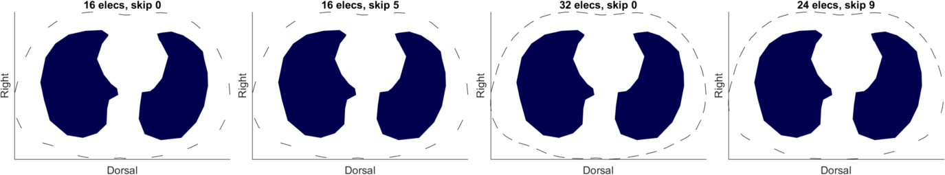
Figure: The four different configurations electrode / skip configurations used in the analysis.

Generating EIT voltage measurements and noise

% generate noisy EIT voltage measurements 
% $ Id:  $

for ii = 1:length(imgs)
    imgs{ii}.elem_data = imgs{ii}.elem_data1;
    vh{ii} = fwd_solve(imgs{ii});
    imgs{ii}.elem_data = imgs{ii}.elem_data2;
    vi{ii} = fwd_solve(imgs{ii});    
end

% generate additive white Gaussian noise
NOISE_N_REALIZATIONS = 1E3;
NOISE_AMPLITUDE = 5E-3;
noise = NOISE_AMPLITUDE * randn(32*32, NOISE_N_REALIZATIONS);

Visualizing noise performance

• Gauss-Newton reconstruction
• GREIT reconstruction

% create reconstruction models and select hyperparameter with different approaches
% $Id: noise_performance_03.m 5760 2018-05-20 10:52:41Z aadler $
if ~exist('rms'); rms = @(n,dim) sqrt(mean(n.^2,dim)); end % define @rms if toolbox not avail

for recon_approach = {'GREIT','GN'}

   switch recon_approach{1}
      case 'GREIT';
         lambda_sel_approach = {'NF', 'SNR', 'LCC', 'GCV'};
         imdl_creation_fun = @(img, opts, lambda) mk_GN_model(img, opts, lambda);    
      case 'GN';
         lambda_sel_approach = {'NF', 'SNR'};
         imdl_creation_fun = @(img, opts, lambda) mk_GREIT_model(img, 0.2, lambda, opts);
      otherwise; error('unspecified recon_approach');
   end
    
   clf;
   for jj = 1:length(lambda_sel_approach)
       for ii = 1:length(imgs)
           subplot(length(lambda_sel_approach), 4, ii + (jj-1)*length(imgs));
           
           opts = [];
           opts.img_size = [32 32];
           switch(lambda_sel_approach{jj})
               case 'NF'   % fixed noise figure
                   lambda = [];    
                   opts.noise_figure = 0.5;    
               case 'SNR'  % fixed image SNR as suggested by Braun et al. 
                   lambda = 1;  % lambda is used as initial weight to find the appropriate SNR
                                % this is an arbitrary initial guess to avoid non-convergence
                   opts.image_SNR = imdl{1,1}.SNR;   % same as NF=0.5 for 16 elecs adjacent
               case 'LCC'  % LCC: L-curve criterion
                   lambda = 1; % lambda will be selected further below
               case 'GCV'  % GCV: generalized-cross validation
                   lambda = 1; % lambda will be selected further below
               otherwise
                   error(['Unknown hyperparameter selection approach: ', lambda_sel_approach(jj)]);
           end
           
           % create reconstruction framework
           imdl{jj, ii} = imdl_creation_fun(mk_image(rmdls{ii},1), opts, lambda);
           imdl{jj, ii}.fwd_model.name = imgs{ii}.fwd_model.name;
           
           % add noise to inhomogeneous conductivity change
           vn = repmat(vi{ii}.meas, 1, size(noise,2)) + noise(1:length(vi{ii}.meas), :);
           
           if strcmp(lambda_sel_approach{jj}, 'LCC') || strcmp(lambda_sel_approach{jj}, 'GCV')
               % use simulated noisy data to choose hyperparameter either with:
               % LCC: L-curve criterion
               % GCV: generalized-cross validation
               lambdas = calc_lambda_regtools(imdl{jj, ii}, vh{ii}.meas, vn, lambda_sel_approach{jj});
               imdl{jj, ii}.hyperparameter.value = median(lambdas);
           end
           
           % calulate image SNR for each approach
           imdl{jj, ii}.SNR = calc_image_SNR(imdl{jj, ii});
           
           % perform image reconstruction
           imgr{jj, ii} = inv_solve(imdl{jj, ii}, vh{ii}.meas, vn);
                   
           % calulate temporal RMS image as in Braun et al., 2017, IEEE TBME        
           trmsa{jj, ii} = imgr{jj, ii};
           trmsa{jj, ii}.elem_data = rms(trmsa{jj, ii}.elem_data, 2);
           % normalize to maximal amplitude
           norm_value = max(trmsa{jj, ii}.elem_data);
           trmsa{jj, ii}.elem_data = trmsa{jj, ii}.elem_data / norm_value;
           imgr{jj, ii}.elem_data = imgr{jj, ii}.elem_data / norm_value;
           % force displaying values in range [0 1]
           trmsa{jj, ii}.calc_colours.clim = 0.5;
           trmsa{jj, ii}.calc_colours.ref_level = 0.5;
           trmsa{jj, ii}.calc_colours.cmap_type = 'greyscale';
           imgr{jj, ii}.calc_colours.clim = 1;
           imgr{jj, ii}.calc_colours.ref_level = 0;
           
           % show tRMSA image for each configuration
           h = show_fem(trmsa{jj, ii}, 1);
           set(h, 'edgecolor', 'none');        
           title([num2str(ii, '(%01d)'), ' ', lambda_sel_approach{jj}, ': ', imdl{jj, ii}.fwd_model.name]);
           set(gca, 'ytick', [], 'xtick', []);
           if ii == 1
               ylabel({['(', char(double('a')+jj-1), ') ', lambda_sel_approach{jj}], 'Right'});
           else
               ylabel('Right');
           end
           xlabel({'Dorsal', sprintf('SNR = %03.2d, \\lambda = %03.2d', imdl{jj, ii}.SNR, imdl{jj, ii}.hyperparameter.value)});
       end
   end
    
   opt.resolution = 200;
   opt.vert_space = 20;
   opt.pagesize   = [16,8];
   switch recon_approach{1}
      case 'GREIT'; print_convert('np_trmsa_GREIT.png',opt)
      case 'GN';    print_convert('np_trmsa_GN.png',opt);
      otherwise; error('unspecified recon_approach');
   end
end %for recon_approach = {'GREIT','GN'}

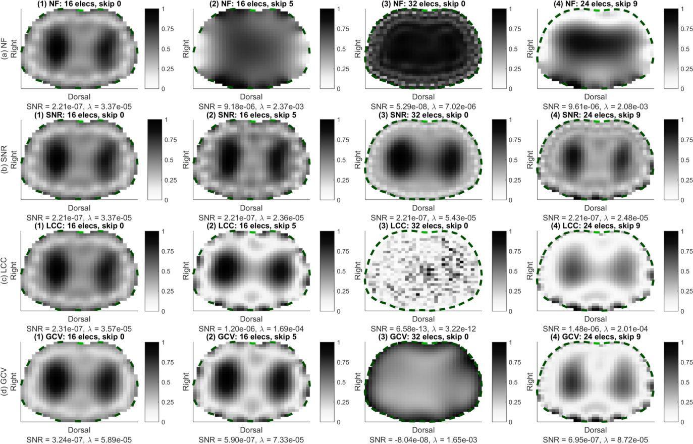
Figure: Gauss Newton reconstruction: temporal RMS amplitude (TRMSA) images of the same conductivity change in the lungs with identical noise for different measurement configurations (1) to (4) and different hyperparameter selection approaches: (a) a fixed noise figure (NF = 0.5), (b) a fixed SNR = 2.21E-07 (equal to NF = 0.5 for the 1st configuration), (c) L-curve criterion (LCC), and (d) generalized cross-validation (GCV).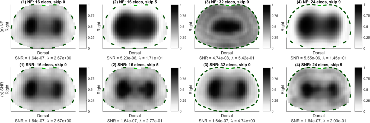

Figure: GREIT reconstruction: temporal RMS amplitude (TRMSA) images of the same conductivity change in the lungs with identical noise for different measurement configurations (1) to (4) and different hyperparameter selection approaches: (a) a fixed noise figure (NF = 0.5), and (b) a fixed SNR = 2.21E-07 (equal to NF = 0.5 for the 1st configuration).

Last Modified: $Date: 2018-05-20 06:55:01 -0400 (Sun, 20 May 2018) $ by $Author: aadler $