EIDORS: Electrical Impedance Tomography and Diffuse Optical Tomography Reconstruction Software

Hosted by

Electrode movement reconstruction for simulated 3D data

% Simulate 3D movement $Id: move_3d01.m 4059 2013-05-24 11:43:38Z bgrychtol $

noiselev = .1;
movement = 2;

% Generate eidors 3D finite element model
mdl3dim = mk_common_model( 'n3r2', [16 2]);
mdl3dim.fwd_model.nodes(:,3) = mdl3dim.fwd_model.nodes(:,3)/3;

img = mk_image(mdl3dim);
vh = fwd_solve( img );

load('datacom.mat','A','B');
img.elem_data(A) = 1.2; 
img.elem_data(B) = 0.8;
node0 = img.fwd_model.nodes;  % Node variable before movement
node1 = node0;                % Node variable after movement
z_axis = node1(:,3);

exaggeration = 10;
movement= 0.01*movement;
% Do a 3D twist - exaggerated for clearer illustration of distortion
node1(:,1) = node0(:,1).*(1 + exaggeration*movement*z_axis);
node1(:,2) = node0(:,2).*(1 + exaggeration*movement*(1-z_axis));

img.fwd_model.nodes = node1;
show_fem( img );
xlabel('x'); ylabel('y');
view(-44,22)

print_convert  move_3d01.png '-density 75'

% Do a 3D twist - we'll actually use this one
centre = 1- movement/2;
node1(:,1) = node0(:,1).*(centre + movement*z_axis);
node1(:,2) = node0(:,2).*(centre + movement*(1-z_axis));

% Solve inhomogeneous forward problem with movements and normal noise.
img.fwd_model.nodes = node1;
vi = fwd_solve( img );
noise = noiselev*std( vh.meas - vi.meas )*randn( size(vi.meas) );
vi.meas = vi.meas + noise;
move = node1 - node0;

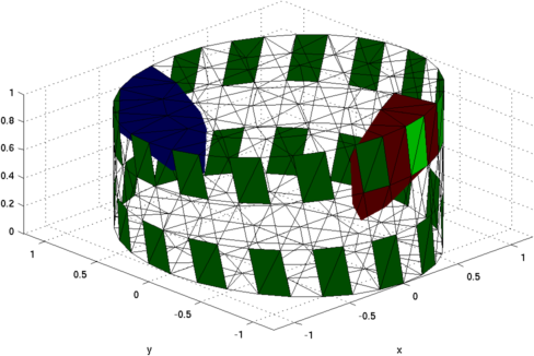
Figure: Illustration of the deformation of the 3D model (exaggerated 10x).

% Reconstruct 3D movement $Id: move_3d02.m 4839 2015-03-30 07:44:50Z aadler $

img3dim= img;

mdl3dim.RtR_prior = 'prior_laplace';
mdl3dim.hyperparameter.value = .05;

% Show slices of 3D model with true movement vectors
subplot(1,3,1);
img3dim.elem_data = img3dim.elem_data - 1;
img3dim.calc_colours.backgnd=[.8 .8 .9];
show_slices_move( img3dim, move );

% Inverse solution of data without movement consideration
img3dim= inv_solve(mdl3dim, vh, vi);
img3dim.calc_colours.backgnd=[.8 .8 .9];
subplot(1,3,2)
show_slices_move( img3dim );

% This is also available by this code:
% mdlM = select_imdl(mdl3dim, {'Elec Move GN'});

% Inverse solution of data with movement consideration
move_vs_conduct = 20;  % Movement penalty (symbol mu in paper)

mdlM = mdl3dim;
mdlM.fwd_model.jacobian = @jacobian_movement;

mdlM.RtR_prior = @prior_movement;

mdlM.prior_movement.parameters = move_vs_conduct;

% Solve inversglobale problem and show slices
imgM = inv_solve(mdlM, vh, vi);
imgM.calc_colours.backgnd=[.8 .8 .9];
subplot(1,3,3)
show_slices_move( imgM );
print_convert  move_3d02.png '-density 100'

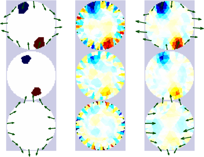
Figure: Inverse solutions of the problem above. Each column shows three cross-sectional slices of the model. Forward problem with true electrode movement (scaled 10x) (left column). Inverse solution without movement compensation (centre column) and with movement estimation and compensation (scaled 10x) (right column).