EIDORS: Electrical Impedance Tomography and Diffuse Optical Tomography Reconstruction Software

Hosted by

Electrode movement reconstruction for simulated 2D data

% Generate simulation data without noise and standard reconstruction
% Create circular FEM - creates a eidors_mdl type inv_model.
mdlc = mk_common_model('c2c');

f_img = mk_image( mdlc, 1);
vh = fwd_solve( f_img );

% Hard coded values here represent local inhomogeneities
f_img.elem_data([75,93,94,113,114,136]) = 1.2;
f_img.elem_data([105,125,126,149,150,174]) = 0.8;

% Simulate node movements - shrink x, stretch y by 1% of model diameter
% node0 before, node1 after movement

movement = [1-0.01 0; 0 1+0.01];
node0 = f_img.fwd_model.nodes;
node1 = node0*movement;
f_img.fwd_model.nodes = node1;

% Solve inhomogeneous forward problem with movements and normal noise
% 1% of standard deviation of signal
vi = fwd_solve( f_img );
move = node1 - node0;

% Plot FEM with conductivities and movement vectors.
show_fem_move( f_img, move, 20 );
print_convert move_2d01.png '-density 75'

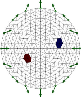
Figure: Forward solution of a 2D model where the boundary was changed between measurements. The arrows show how the electrodes were displaced (scaled 20x).

% Generate eidors planar finite element model
mdl2dim = mk_common_model('b2c');
mdl2dim.hyperparameter.value= 0.1;

clim= .088;

% Solve inverse problem for mdl2dim eidors_obj model.
img2dim = inv_solve(mdl2dim, vh, vi);
img2dim.calc_colours.clim= clim;
img2dim.calc_colours.backgnd= [.9,.9,.9];

% Plot results for each algorithm
subplot(1,2,1);
show_fem_move(img2dim);
img2dim.calc_colours.cb_shrink_move = [0.5,1.0,.02];
eidors_colourbar(img2dim);

% Set eidors_obj hyperparameter member.
mdlM = mdl2dim;

mdlM.fwd_model.jacobian = @jacobian_movement;
mdlM.RtR_prior =          @prior_movement;
mdlM.prior_movement.parameters = sqrt(1e2/1); 

% Solve inverse problem for mdlM eidors_obj model.
imgM = inv_solve(mdlM, vh, vi);
imgM.calc_colours.clim= clim;
imgM.calc_colours.backgnd= [.9,.9,.9];

% Plot results for each algorithm
subplot(1,2,2);
show_fem_move(imgM);
imgM.calc_colours.cb_shrink_move = [0.5,0.9,.02];
eidors_colourbar(imgM);

print_convert move_2d02.png

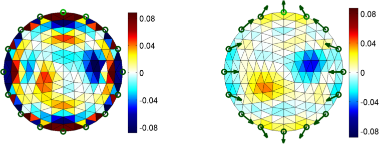
Figure: Inverse solutions of the problem above. Left image shows image reconstruction without movement correction, and right image shows reconstruction with estimated movement corrections shown by green arrows (scaled 20x).