EIDORS: Electrical Impedance Tomography and Diffuse Optical Tomography Reconstruction Software

Hosted by

Iterative Gauss Newton reconstruction in 3D

% Create simulation data $Id: basic_iterative01.m 5524 2017-06-07 20:17:16Z aadler $

% 3D Model
imdl_3d= mk_common_model('n3r2',[16,2]);
show_fem(imdl_3d.fwd_model);

sim_img= mk_image( imdl_3d.fwd_model, 1);

% set homogeneous conductivity and simulate
homg_data=fwd_solve( sim_img );

% set inhomogeneous conductivity and simulate
sim_img.elem_data([390,391,393,396,402,478,479,480,484,486, ...
                   664,665,666,667,668,670,671,672,676,677, ...
                   678,755,760,761])= 10;
sim_img.elem_data([318,319,321,324,330,439,440,441,445,447, ...
                   592,593,594,595,596,598,599,600,604,605, ...
                   606,716,721,722])= 0.1;
inh_data=fwd_solve( sim_img );


slice_posn = [inf,inf,2.2,1,1; ...
              inf,inf,1.5,1,2;
              inf,inf,0.8,1,3];
show_slices(sim_img,slice_posn);

print -r75 -dpng basic_iterative01a.png

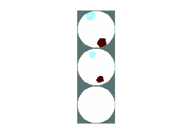
Figure: Three slices of a simple 3D shape to image (from top to bottom, at z=2.2, z=1.5, z=0.8)

Reconstruction with different iterations

% Reconstruct images $Id: basic_iterative02.m 5524 2017-06-07 20:17:16Z aadler $

% Set reconstruction inv_solve_gn
imdl_3d.solve= @inv_solve_gn;
imdl_3d.RtR_prior= @prior_laplace;
imdl_3d.hyperparameter.value= .01;
imdl_3d.inv_solve_gn.return_working_variables = 1;
iter_res = @(img) [size(img.inv_solve_gn.r,1)-1, img.inv_solve_gn.r(end,1)];


% Number of iterations and tolerance (defaults)
imdl_3d.inv_solve_gn.max_iterations = 1;

%Add 30dB SNR noise to data
noise_level= std(inh_data.meas - homg_data.meas)/10^(30/20);
noise_level=0;
inh_data.meas = inh_data.meas + noise_level* ...
                randn(size(inh_data.meas));

% Reconstruct Images: 1 Iteration
subplot(131)
imdl_3d.inv_solve_gn.max_iterations = 1;
rec_img= inv_solve(imdl_3d, homg_data, inh_data);
show_slices(rec_img,slice_posn);
title(sprintf('iter=%d resid=%5.3f',iter_res(rec_img)));


% Reconstruct Images: 2 Iterations
subplot(132)
imdl_3d.inv_solve_gn.max_iterations = 2;
rec_img= inv_solve(imdl_3d, homg_data, inh_data);
show_slices(rec_img,slice_posn);
title(sprintf('iter=%d resid=%5.3f',iter_res(rec_img)));

% Reconstruct Images: 5 Iterations -- but stops at 4 (not improving)
subplot(133)
imdl_3d.inv_solve_gn.max_iterations = 5;
rec_img= inv_solve(imdl_3d, homg_data, inh_data);
show_slices(rec_img,slice_posn);
title(sprintf('iter=%d resid=%5.3f',iter_res(rec_img)));


print -r75 -dpng basic_iterative02a.png

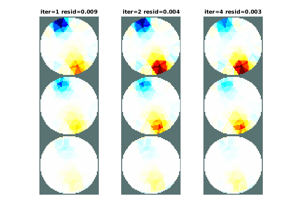
Figure: Images from GN reconstructions. From left to right: 1 iteration, 2 iterations, 4 iterations. Little difference is seen in this case, mostly because this is a difference imaging problem with small contrasts.

Residuals

% Plot residuals $Id: basic_iterative03.m 5558 2017-06-18 17:21:58Z aadler $
subplot(211);
r = rec_img.inv_solve_gn.r;
k = size(r,1)-1;

x = 1:(k+1); % k+1 => look at the solve after last iteration
y = r(x, :);
y = y ./ repmat(max(y,[],1),size(y,1),1) * 100;
plot(x-1, y, 'o-', 'linewidth', 2, 'MarkerSize', 10);
title('residuals');
axis tight;
ylabel('residual (% of max)');
xlabel('iteration');
set(gca, 'xtick', x);
set(gca, 'xlim', [0 max(x)-1]);
legend('residual','meas. misfit','prior misfit');
legend('Location', 'East');
print_convert basic_iterative03a.png

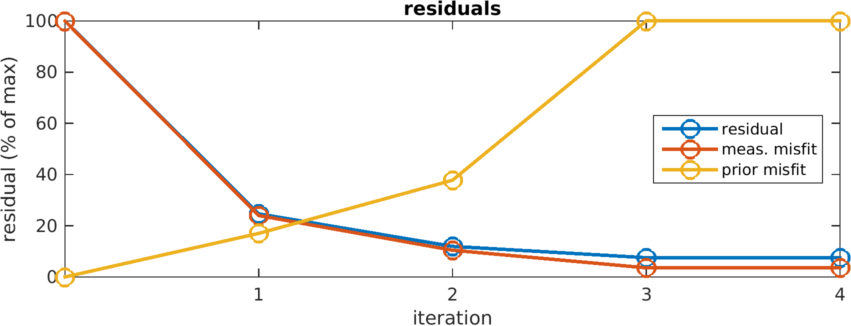
Figure: Residals and misfit curves vs iteration

>>rec_img.inv_solve_gn.r(:,1)
ans =
    0.0365
    0.0090
    0.0043
    0.0028
    0.0028