EIDORS: Electrical Impedance Tomography and Diffuse Optical Tomography Reconstruction Software

Hosted by

Absolute Imaging: Non-Linear Gauss Newton Image Reconstruction

% Create model for Absolute Imaging
% Based on example from Stephen Murphy
% $Id: tutorial151a.m 2784 2011-07-14 21:25:40Z bgrychtol $

load tutorial151_model.mat

% Create Simulation Model
sim_img= eidors_obj('image', 'Simulation Image');
sim_img.fwd_model= simmdl;

backgnd= .02; 
sim_img.elem_data= backgnd*ones(size(simmdl.elems,1),1);
sim_img.elem_data(target1)= backgnd*2;
sim_img.elem_data(target2)= backgnd/4;

clf;
axes('position',[.1,.1,.65,.8]);
   show_fem(sim_img); view(-33,20);
axes('position',[.8,.1,.15,.8]);
   show_slices(sim_img,5);

print_convert tutorial151a.png '-density 75'

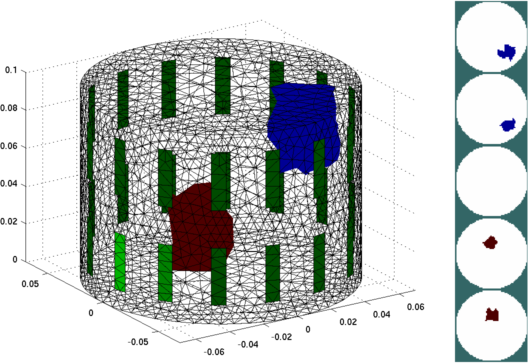
Figure: Left: Simulation Model (20951 elements), showing a non-conductive (blue) and conductive (red) target Right: Simulation Model viewed as equispaced horizontal slices

% Simulate data for difference and absolute imaging
% $Id: tutorial151b.m 2784 2011-07-14 21:25:40Z bgrychtol $

% Create homogeneous simulation Model
backgnd= .02; 
sim_img.elem_data= backgnd*ones(size(simmdl.elems,1),1);
v_homg= fwd_solve(sim_img);

% Create target simulation Model
sim_img.elem_data(target1)= backgnd*2;
sim_img.elem_data(target2)= backgnd/4;
v_targ= fwd_solve(sim_img);

clf; subplot(211);
plot([v_homg.meas, v_targ.meas]);
print_convert tutorial151b.png '-density 75'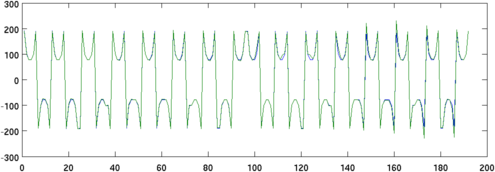

Figure: Green Homogeneous measurements, Blue Target measurements,

% Difference imaging result
% $Id: tutorial151c.m 4839 2015-03-30 07:44:50Z aadler $

% imdl is loaded from file tutorial151_model.mat
imdl.reconst_type= 'difference';
imdl.solve=        @inv_solve_diff_GN_one_step;
imdl.jacobian_bkgnd.value= backgnd;
imdl.hyperparameter.value= .1;
img_diff= inv_solve(imdl, v_homg, v_targ);

clf;
axes('position',[.1,.1,.65,.8]);
   show_fem(img_diff); view(-33,20);
axes('position',[.8,.1,.15,.8]);
   show_slices(img_diff,5);

print_convert tutorial151c.png '-density 75'

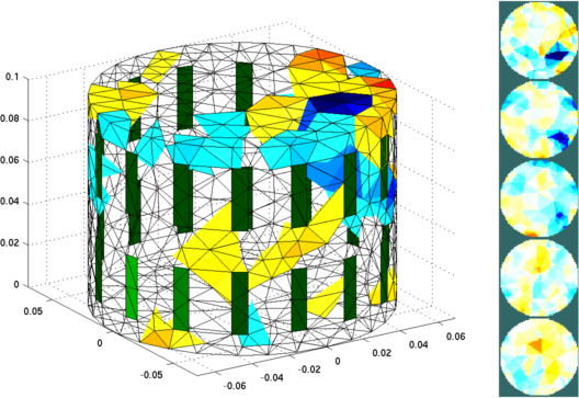
Figure: Left: Reconstructed Image (2266 elements), showing a non-conductive (blue) and conductive (red) target Right: Simulation Model viewed as equispaced horizontal slices

function img= tutorial151_nonlinearGN( inv_model, data )
% TUTORIAL151_NONLINEARGN Non-Linear EIT Inverse
% img        => output image (or vector of images)
% inv_model  => inverse model struct
% data       => measurement data
% $Id: tutorial151_nonlinearGN.m 3661 2012-11-20 21:18:01Z bgrychtol $

fwd_model= inv_model.fwd_model;

img= eidors_obj('image','Solved by tutorial151_nonlinearGN');
img.fwd_model= fwd_model;
sol= inv_model.tutorial151_nonlinearGN.init_backgnd * ...
     ones(size(fwd_model.elems,1),1);

RtR = calc_RtR_prior( inv_model );
hp2  = calc_hyperparameter( inv_model )^2;

factor= 0; norm_d_data= inf;
for iter= 1:inv_model.parameters.max_iterations
   img.elem_data= sol;
   simdata= fwd_solve( img );

   d_data= data - simdata.meas;
   prev_norm_d_data= norm_d_data; norm_d_data= norm(d_data); 
   eidors_msg('tutorial151_nonlinearGN: iter=%d err=%f factor=%f', ...
           iter,norm_d_data, factor, 2);

   if prev_norm_d_data - norm_d_data < inv_model.parameters.term_tolerance
      break;
   end
   
   J = calc_jacobian( img);
   delta_sol = (J.'*J + hp2*RtR)\ (J.' * d_data);
   factor= linesearch(img, data, sol, delta_sol, norm_d_data);
   sol = sol + factor*delta_sol;
end

   img.elem_data= sol;

% Test several different factors to see which minimizes best
function factor= linesearch(img, data, sol, delta_sol, norm_d_data);
   facts= [0, logspace(-3,0,19)];  
   norms= norm_d_data;
   for f= 2:length(facts);
      img.elem_data= sol + facts(f)*delta_sol;
      simdata= fwd_solve( img );
      norms(f)= norm(data - simdata.meas);
   end
   ff= find(norms==min(norms));
   factor= facts(ff(end));

% Absolute imaging result
% $Id: tutorial151d.m 4839 2015-03-30 07:44:50Z aadler $

% imdl is loaded from file tutorial151_model.mat
imdl.reconst_type= 'static';
imdl.solve=        @tutorial151_nonlinearGN;
imdl.parameters.term_tolerance= 1e-5;
imdl.parameters.max_iterations= 10;
% special parameter for this model
imdl.tutorial151_nonlinearGN.init_backgnd= backgnd;

imdl.hyperparameter.value= 2;
img_diff= inv_solve(imdl, v_targ);

clf;
axes('position',[.1,.1,.65,.8]);
   show_fem(img_diff); view(-33,20);
axes('position',[.8,.1,.15,.8]);
   show_slices(img_diff,5);

print_convert tutorial151d.png '-density 75'

>> tutorial151d;
EIDORS:[ inv_solve:nonlinear Gauss Newton for absolute imaging demo ]
EIDORS:[ tutorial151_nonlinearGN: iter=1 err=52.820965 factor=0.000000 ]
EIDORS:[ tutorial151_nonlinearGN: iter=2 err=11.468709 factor=0.014678 ]
EIDORS:[ tutorial151_nonlinearGN: iter=3 err=7.208743 factor=0.014678 ]
EIDORS:[ tutorial151_nonlinearGN: iter=4 err=2.284559 factor=0.031623 ]
EIDORS:[ tutorial151_nonlinearGN: iter=5 err=0.850762 factor=0.014678 ]
EIDORS:[ tutorial151_nonlinearGN: iter=6 err=0.599933 factor=0.021544 ]
EIDORS:[ tutorial151_nonlinearGN: iter=7 err=0.519560 factor=0.031623 ]
EIDORS:[ tutorial151_nonlinearGN: iter=8 err=0.341341 factor=0.068129 ]
EIDORS:[ tutorial151_nonlinearGN: iter=9 err=0.307938 factor=0.014678 ]
EIDORS:[ tutorial151_nonlinearGN: iter=10 err=0.262837 factor=0.068129 ]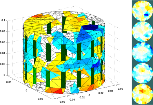

Figure: Left: Reconstructed absolute Image (2266 elements), showing a non-conductive (blue) and conductive (red) target Right: Simulation Model viewed as equispaced horizontal slices