|
|
EIDORS: Electrical Impedance Tomography and Diffuse Optical Tomography Reconstruction Software |
|
EIDORS
(mirror) Main Documentation Tutorials − Image Reconst − Data Structures − Applications − FEM Modelling − GREIT − Old tutorials − Workshop Download Contrib Data GREIT Browse Docs Browse SVN News Mailing list (archive) FAQ Developer
Hosted by |
GREIT Reconstruction in 3D −This tutorial shows how to reproduce the 2×16 electrode and 1×32 electrode belt images from the following paper:Grychtol et al, Focusing EIT reconstructions using two electrode planes p. 17 Conf. EIT 2017, Dartmouth, NH, USA, June 21−24, 2017.Data for this tutorial are available here: horse-breathing3D2D.mat 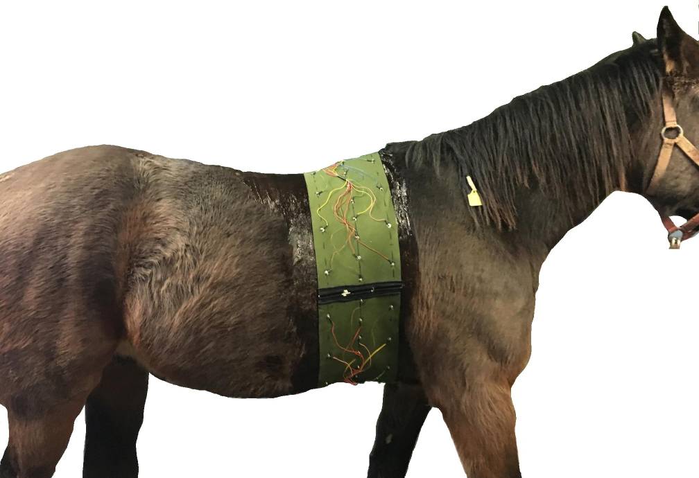
Figure: Standing horse with an electrode belt allowing 2×16 electrode and 1×32 electrode belt EIT data recording GREIT 3D softwareCode for Reconstruction using GREIT is in EIDORS v3.9.1. If you have an older version (EIDORS v3.9) you will need the following two files: This code is also very slow to calculate. The actual reconstruction is fast. There are numerous improvements possible, and they're being worked on.3D FEM for 1×32 electrode belt
% Model of 32x1 electrode belt
fmdl= ng_mk_ellip_models([4,0.8,1.1,.5],[32,2.0],[0.05]);
% Swisstom BBVet stimulation pattern
skip4 = {32,1,[0,5],[0,5],{'no_meas_current_next1'},1};
[fmdl.stimulation,fmdl.meas_select] = mk_stim_patterns(skip4{:});
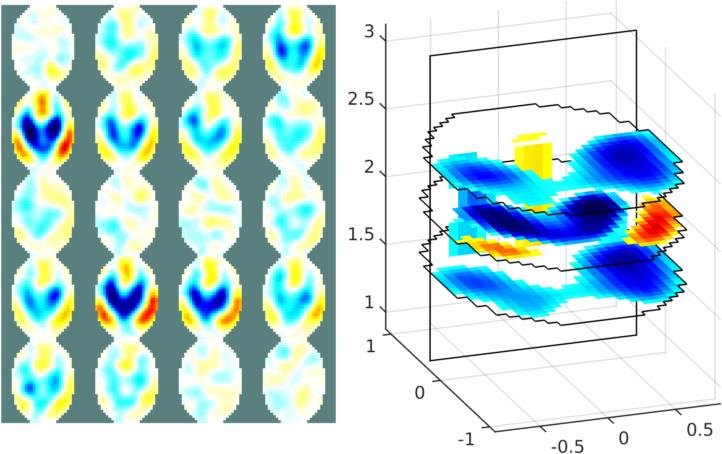
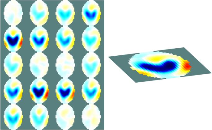
3D GREIT reconstruction with 1×32 electrode beltvopt.imgsz = [32 32]; vopt.square_pixels = true; vopt.zvec = linspace(-1,1,10)*1.125 + 2; vopt.save_memory = 1; opt.noise_figure = 1.0; % GREIT 3D with a 1x32 electrode layout [imdl,opt.distr] = GREIT3D_distribution(fmdl, vopt); imdl2a= mk_GREIT_model(imdl, 0.20, [], opt); 2D GREIT reconstruction with 1×32 electrode belt% 2D GREIT model clear opt; opt.imgsz = [32 32]; opt.square_pixels = true; opt.noise_figure = 0.5; img = mk_image(fmdl,1); imdl2b= mk_GREIT_model(img, 0.25, [], opt); 3D FEM for 2×16 electrode belt
fmdl= ng_mk_ellip_models([4,0.8,1.1,.5],[16,1.7,2.3],[0.05]);
[fmdl.stimulation,fmdl.meas_select] = mk_stim_patterns(skip4{:});

% "Square" electrode layout
idx = reshape(1:32,2,[])';
idx(2:2:end,:) = fliplr(idx(2:2:end,:));
extraflip= [4:12]; % This belt was made slightly differently
idx(extraflip,:) = fliplr(idx(extraflip,:));
fmdl.electrode(idx) = fmdl.electrode(:);
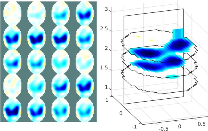
3D GREIT reconstruction with 2×16 electrode beltvopt.imgsz = [32 32]; vopt.square_pixels = true; vopt.zvec = linspace(-1,1,10)*1.125+2; vopt.save_memory = 1; opt.noise_figure = 1.0; % GREIT 3D with 2x16 electrode belt [imdl,opt.distr] = GREIT3D_distribution(fmdl, vopt); imdl3= mk_GREIT_model(imdl, 0.20, [], opt); Load data and reconstruct imagesUsing data: horse-breathing3D2D.mat
load horse-breathing3D2D.mat

for i=1:3; switch i;
   case 1; imdl = imdl3;  vv= horse3d; % 2 planes, 3D GREIT
   case 2; imdl = imdl2a; vv= horse2d; % 1 plane, 3D GREIT
   case 3; imdl = imdl2b; vv= horse2d; % 1 plane, 2D GREIT
   end

   img = inv_solve(imdl,vv(:,1),vv(:,2:end));
   img.calc_colours.ref_level = 0;
   subplot(121);
   show_slices(img,[inf,inf,2]);

   subplot(122);
   img.elem_data = img.elem_data(:,6);
   if i<3; show_3d_slices(img,[1.6,2.0,2.4],[],[0.4]);
   else;   show_slices(img);
   end;    view(-20,20);

   print_convert(sprintf('GREIT3D_horse06%c.jpg',64+i));
end
Figure: Reconstructed images of two tidal breaths for two different electrode belts Last Modified: $Date: 2018-06-14 10:44:51 -0400 (Thu, 14 Jun 2018) $ by $Author: aadler $ |