EIDORS: Electrical Impedance Tomography and Diffuse Optical Tomography Reconstruction Software

Hosted by

GREIT evaluation: Make simulation data (3D)

Prepare simulation data: phantom data

% simulate radial movement $Id: simulation_3d_test00.m 2726 2011-07-13 20:07:48Z aadler $
use_3d_model = 1;

if use_3d_model;
   fmdl= ng_mk_cyl_models([30,15,1],[16,15],[0.5]);
else;
   imdl = mk_common_model('f2d3c',16); fmdl= imdl.fwd_model;
end

stim_pat = mk_stim_patterns(16,1,'{ad}','{ad}', {'no_meas_current'}, 1);

fmdl.stimulation = stim_pat;

% simulate radial movement $Id: simulation_3d_test01.m 2726 2011-07-13 20:07:48Z aadler $

if exist('sim_radmove_homog.mat','file')
   load sim_radmove_homog.mat vh vi xyzr_pt
else
   params= [0.9,0.05,0.5,0.5]; %max_posn, targ_rad, z_0, z_t
   stim_pat = mk_stim_patterns(16,1,'{ad}','{ad}', {'no_meas_current'}, 1);
   if use_3d_model;
      [vh,vi,xyzr_pt]= simulate_3d_movement(500, fmdl, params, @simulation_radmove);
      xyzr_pt= xyzr_pt([2,1,3,4],:)/15; %Change: mdl geometry at 90 deg; radius is 15
   else;
      [vh,vi,xyzr_pt]= simulate_2d_movement(500, fmdl, params, @simulation_radmove);
      xyzr_pt = [-1,0,0;0,1,0;0,0,0;0,0,1]*xyzr_pt;
   end

   save sim_radmove_homog vh vi xyzr_pt
end

function [xp,yp,zp]= simulation_radmove(f_frac, radius, z0,zt);
% Radial Movement - $Id: simulation_radmove.m 2700 2011-07-13 12:26:06Z aadler $  
   rp= f_frac*radius; 
   cv= 2*pi*f_frac * 73;
   xp= rp * cos(cv);
   yp= rp * sin(cv);
   if nargin==4; zp = mean([zt,z0]); else; zp= 0; end

% Show simulated positions $Id: simulation_3d_test02.m 2785 2011-07-14 21:34:08Z aadler $
clf; show_fem(fmdl)
crop_model(gca, inline('x-z<-15','x','y','z'))
      view(-90,20)

hold on
[xs,ys,zs]=sphere(10); spclr= [0,.5,.5];
for i=1:1:size(xyzr_pt,2);
   xp=15*xyzr_pt(1,i); yp=15*xyzr_pt(2,i); zp=15*xyzr_pt(3,i); rp=15*xyzr_pt(4,i);
   hh=surf(rp*xs+xp, rp*ys+yp, rp*zs+zp);
   set(hh,'EdgeColor',[0,.4,.4],'FaceColor',[0,.8,.8]);
   hh=text(xp,yp,zp+1,num2str(i)); 
   set(hh,'FontSize',7,'FontWeight','bold','HorizontalAlignment','center');
end
hold off

print_convert simulation_3d_test02a.png 

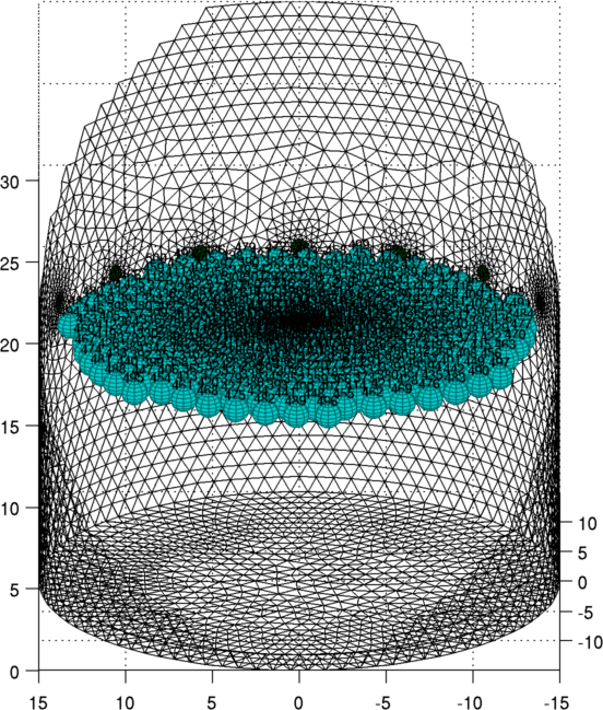
Figure: Position and size of simulated conductive targets in medium