EIDORS: Electrical Impedance Tomography and Diffuse Optical Tomography Reconstruction Software

Hosted by

GREIT evaluation: Make simulation data (2D)

Prepare simulation data: create phantom model in 2D

% create model $Id: simulate_2d_test01.m 3828 2013-04-13 14:20:17Z bgrychtol $

% Model parameters
n_elec= 16;
n_nodes= 2000;

% Create electrodes
refine_level=4; %electrode refinement level
elec_width= .1;
z_contact = 0.01;
% elect positions
th=linspace(0,2*pi,n_elec(1)+1)';th(end)=[];
elec_posn= [sin(th),cos(th)];
[elec_nodes, refine_nodes] = dm_mk_elec_nodes( elec_posn, elec_width, refine_level);

% Define circular medium
fd=inline('sum(p.^2,2)-1','p');
bbox = [-1,-1;1,1];
smdl = dm_mk_fwd_model( fd, [], n_nodes, bbox, elec_nodes, refine_nodes, z_contact);
smdl = mdl_normalize(smdl,0); 

% simulate homogeneous $Id: simulate_2d_test02.m 3273 2012-06-30 18:00:35Z aadler $

% stimulation pattern: adjacent
stim_pat= mk_stim_patterns(n_elec,1,'{ad}','{ad}',{},1);

smdl.stimulation= stim_pat;
himg= mk_image(smdl,1);

vh= fwd_solve(himg); vh= vh.meas;

Prepare simulation data: create phantom model in 2D

% moving target $Id: simulate_2d_test03.m 3828 2013-04-13 14:20:17Z bgrychtol $

% Create a moving object within the model
trg_rad= 0.05; trs= trg_rad*sin(th); trc= trg_rad*cos(th);
radius= 0.9;
n_sims= 2 ;
contrast= 0.1;

vi=[];
for i= 1:n_sims; 
   f_frac = (i-1)/(n_sims-1);
   cv= 2*pi*f_frac * 73;
   trg_ctr= f_frac*radius*[cos(cv),sin(cv)];

   trg_refine_nodes= [refine_nodes; [ trs+trg_ctr(1), trc+trg_ctr(2) ]];

   tmdl= dm_mk_fwd_model( fd, [], n_nodes, bbox, elec_nodes, trg_refine_nodes, z_contact);
   tmdl.stimulation = stim_pat;
   tmdl = mdl_normalize(tmdl,0);

   % find elements in size target
   mdl_pts = interp_mesh( tmdl );
   ctr_pts = mdl_pts - ones(size(mdl_pts,1),1)*trg_ctr;
   in_trg  =(sum(ctr_pts.^2,2) < trg_rad^2);

   % Create target image object
   timg= mk_image(tmdl, 1 + in_trg*contrast);
   vi_t= fwd_solve(timg);
   vi = [vi, vi_t.meas];
   if     i==1;    show_fem(timg); print -dpng -r60 simulate_2d_test03a.png
   elseif i==150;  show_fem(timg); print -dpng -r60 simulate_2d_test03b.png
   end
end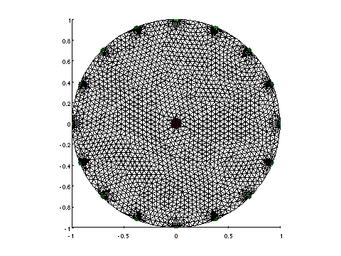

Figure: Position and size of conductive targets in medium