EIDORS: Electrical Impedance Tomography and Diffuse Optical Tomography Reconstruction Software

Hosted by

GREIT software framework

0. Construction of the forward model (fwd_model). This is saved to a file, and must inlude the main EIDORS structures:
   − fwd_model.elems (N_elems×4) - definition of simplices
   − fwd_model.nodes (N_nodes×3) - definition of vertices
   − fwd_model.electrode (N_electrodes) - normally 16, 12 or 8
   − fwd_model.electrode(idx).nodes - nodes in the electrode
   − fwd_model.electrode(idx).z_contact - contact impedance for Complete electrode model
1. Calculation of Jacobian
   based on fwd_model and a reconstruction model using a 32×32 grid which covers the x, y space of the fwd_model.
   Parameter values include the height of the reconstruction grid
2. Calculation of the image prior
   no parameters are required, typically, except for NOSER type priors which require calculation of the Jacobian.
3. Calculation of the reconstruction matrix
   This step involves the inverse step, and calcualtion of the hyperparameter, via an explicit hyperparameter (λ) or via a scheme such as the truncated SVD.
4. Evaluation of the reconstruction matrix
   Each different evaluation figure of metrit is calculated from the reconstruction matrix using a different hyperparameter.

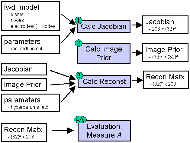
Figure: Conceptual framework for GREIT software

Step 0: forward model

% fwd_model $Id: framework00.m 2684 2011-07-13 08:43:58Z aadler $

fmdl = mk_library_model('cylinder_16x1el_fine');
fmdl.stimulation = mk_stim_patterns(16,1,'{ad}','{ad}',{},1);

subplot(121)
show_fem(fmdl);
view([-5 28]);
crop_model(gca, inline('x+2*z>20','x','y','z'))

subplot(122)
show_fem(fmdl);
view(0,0);
crop_model(gca, inline('y>-10','x','y','z'))
set(gca,'Xlim',[-4,4],'Zlim',[-2,2]+5);

print_convert framework00a.png

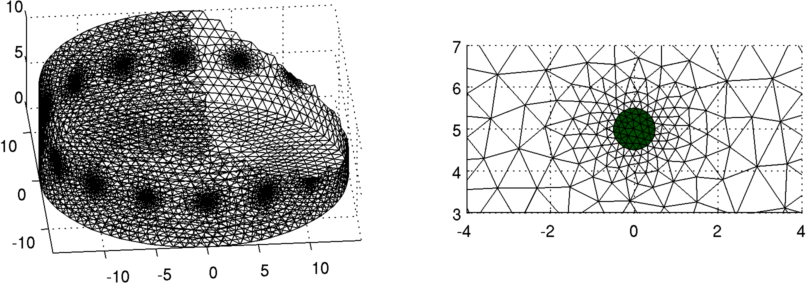
Figure: FEM model of a ring of electrodes as well. Right Refinement of mesh near the electrode.

Step 1: calculate Jacobian

% fwd_model $Id: framework01.m 2684 2011-07-13 08:43:58Z aadler $

fmdl = mk_library_model('cylinder_16x1el_fine');

pixel_grid= 32;
nodes= fmdl.nodes;
xyzmin= min(nodes,[],1);  xyzmax= max(nodes,[],1);
xvec= linspace( xyzmin(1), xyzmax(1), pixel_grid+1);
yvec= linspace( xyzmin(2), xyzmax(2), pixel_grid+1);
zvec= [0.6*xyzmin(3)+0.4*xyzmax(3), 0.4*xyzmin(3)+0.6*xyzmax(3)];

% CALCULATE MODEL CORRESPONDENCES
[rmdl,c2f] = mk_grid_model(fmdl, xvec, yvec, zvec);


% SHOW MODEL CORRESPONDENCE

clf;
show_fem(fmdl);  % fine model
crop_model(gca, inline('x-z<-8','x','y','z'))
hold on
hh=show_fem(rmdl); set(hh,'EdgeColor',[0,0,1]);
hold off

view(-47,18); 

print_convert framework01a.png

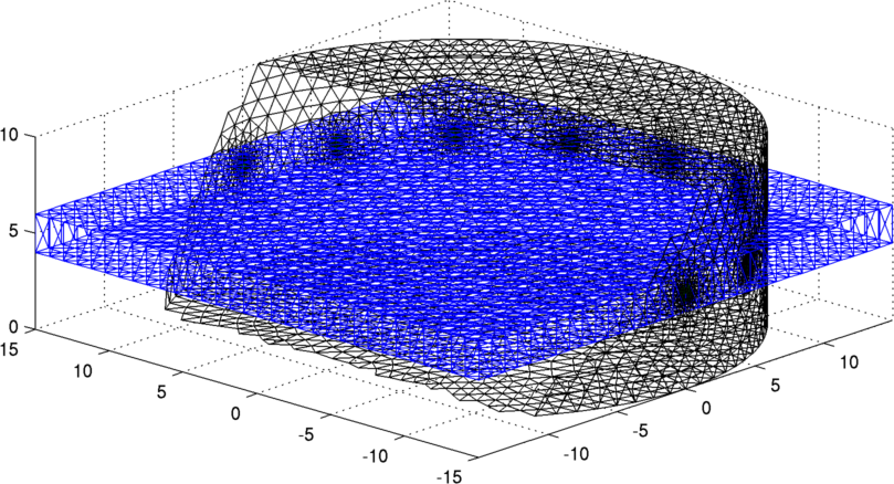
Figure: 3D fine cylindrical mesh and 32×32 reconstruction grid

% fwd_model $Id: framework02.m 3273 2012-06-30 18:00:35Z aadler $

% CALCULATE JACOBIAN AND SAVE IT

img= mk_image(fmdl, 1);
img.fwd_model.coarse2fine = c2f;
img.rec_model= rmdl;

% ADJACENT STIMULATION PATTERNS
img.fwd_model.stimulation= mk_stim_patterns(16, 1, ...
             [0,1],[0,1], {'do_redundant', 'no_meas_current'}, 1);

% SOLVERS
img.fwd_model.system_mat= @system_mat_1st_order;
img.fwd_model.solve=      @fwd_solve_1st_order;
img.fwd_model.jacobian=   @jacobian_adjoint;

J= calc_jacobian(img);

map = reshape(sum(c2f,1),pixel_grid,pixel_grid)>0;
save GREIT_Jacobian_ng_mdl_fine J map

Step 2: calculate image prior

% image prior $Id: framework03.m 1545 2008-07-26 17:33:46Z aadler $
load GREIT_Jacobian_ng_mdl_fine J map

% Remove space outside FEM model
J= J(:,map);
% inefficient code - but for clarity
diagJtJ = diag(J'*J) .^ (0.7);

R= spdiags( diagJtJ,0, length(diagJtJ), length(diagJtJ));

save ImagePrior_diag_JtJ R

Step 3: calculate reconstruction matrix

% reconst $Id: framework04.m 1544 2008-07-26 17:23:52Z aadler $
load ImagePrior_diag_JtJ R
load GREIT_Jacobian_ng_mdl_fine J map

RM = zeros(size(J'));
J = J(:,map);

hp = .3;

RM(map,:)= (J'*J + hp^2*R)\J';

save RM_framework_example RM map

Step 4: test reconstruction matrix

% Test RM $Id: framework05.m 3846 2013-04-16 16:24:32Z aadler $

% EXCLUDE MEASURES AT ELECTRODES
[x,y]= meshgrid(1:16,1:16);
idx= abs(x-y)>1 & abs(x-y)<15;

% LOAD SOME TEST DATA
load iirc_data_2006
v_reference= - real(v_reference(idx,:));
v_rotate   = - real(v_rotate(idx,:));

load RM_framework_example RM map;
clear imgs;for k=1:4;
   dv = v_rotate(:,k*2) - v_reference;
   img = reshape( RM*dv, 32,32); % reconstruction
   img(~map) = NaN;              % background
   imgs(:,:,k) = img;
end

imagesc(reshape(imgs,32,4*32))
axis off; axis equal; colormap(gray(256))
print_convert framework05a.png '-density 75'

Figure: Images of a non-conductive object moving in a tank.