EIDORS: Electrical Impedance Tomography and Diffuse Optical Tomography Reconstruction Software

Hosted by

Compare 3D image reconstructions

The first step is to create a simulation model

% Compare 3D algorithms
% $Id: tutorial130a.m 4051 2013-05-24 09:27:02Z bgrychtol $

imb=  mk_common_model('n3r2',[16 2]);
bkgnd= 1;

% Homogenous Data
img= mk_image(imb.fwd_model, bkgnd);
vh= fwd_solve( img );

% Inhomogenous Data - Load from file 'datacom'
load datacom A B;
img.elem_data(A)= bkgnd*1.2;
img.elem_data(B)= bkgnd*0.8;
clear A B;
vi= fwd_solve( img );

% Add 15dB noise
vi_n= vi; 
vi_n.meas = vi.meas + std(vi.meas - vh.meas)/10^(10/20) ...
                     *randn(size(vi.meas));
sig= sqrt(norm(vi.meas - vh.meas));

subplot(121);
show_fem(img); axis square;

subplot(122);
show_fem(img); axis square;
crop_model([],  inline('y<0','x','y','z'))
view(-51,14);
print_convert('tutorial130a.png', '-density 100')

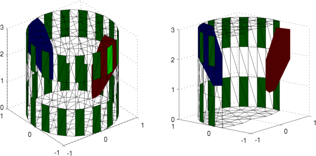
Figure: Simulation image for sample data (two different views)

% Compare 3D algorithms
% $Id: tutorial130b.m 4839 2015-03-30 07:44:50Z aadler $
clear imgr imgn

% Create Inverse Model
inv3d= eidors_obj('inv_model', 'EIT inverse');
inv3d.reconst_type= 'difference';
inv3d.jacobian_bkgnd.value = 1;
inv3d.fwd_model= imb.fwd_model;
inv3d.hyperparameter.value = 0.03; 


% Gauss-Newton Solver
inv3d.solve=       @inv_solve_diff_GN_one_step;

% Tikhonov prior
inv3d.R_prior=     @prior_tikhonov;
imgr(1)= inv_solve( inv3d, vh, vi);
imgn(1)= inv_solve( inv3d, vh, vi_n);

% Laplace prior
inv3d.R_prior=     @prior_laplace;
% inv3d.np_calc_image_prior.parameters= [3 1]; %  deg=1, w=1
imgr(2)= inv_solve( inv3d, vh, vi);
imgn(2)= inv_solve( inv3d, vh, vi_n);

% Andrea Borsic's PDIPM TV solver
inv3d.prior_TV.alpha2 = 1e-5;
inv3d.parameters.max_iterations= 20;
inv3d.parameters.term_tolerance= 1e-3;
inv3d.R_prior=     @prior_TV;
inv3d.solve=       @inv_solve_TV_pdipm;

imgr(3)= inv_solve( inv3d, vh, vi);
imgn(3)= inv_solve( inv3d, vh, vi_n);

% Output image
posn= [inf,inf,2.5,1,1;inf,inf,1.5,1,2;inf,inf,0.5,1,3];
clf;
imgr(1).calc_colours.npoints= 128;
show_slices(imgr, posn);
print_convert('tutorial130b.png', '-density 100')

imgn(1).calc_colours.npoints= 128;
show_slices(imgn, posn);
print_convert('tutorial130c.png', '-density 100')

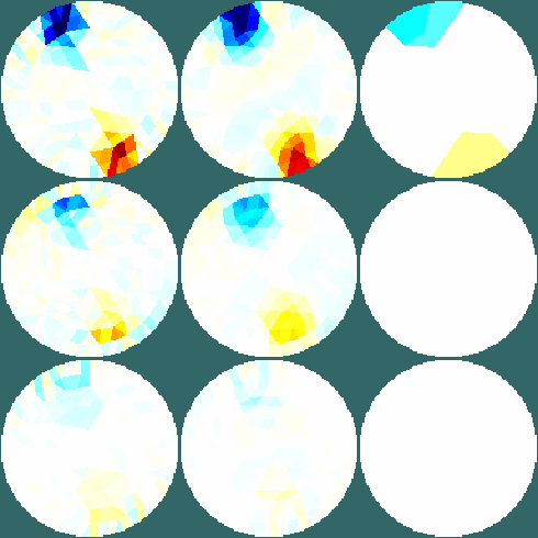
Figure: Images reconstructed with data without noise. Slices are shown at heights of (top to bottom): 1) 2.5, 2) 1.5, 3) 0.5. From Left to Right: 1) One step Gauss-Newton reconstruction (Tikhonov prior) 2) One step Gauss-Newton reconstruction (Laplace filter prior) 3): Total Variation reconstruction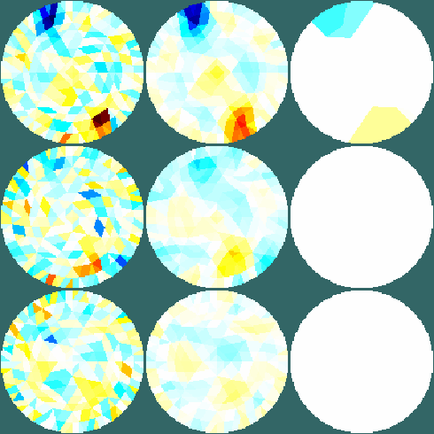

Figure: Images reconstructed with data with 15dB SNR. Slices are shown at heights of (top to bottom): 1) 2.5, 2) 1.5, 3) 0.5. From Left to Right: 1) One step Gauss-Newton reconstruction (Tikhonov prior) 2) One step Gauss-Newton reconstruction (Laplace filter prior) 3): Total Variation reconstruction