EIDORS: Electrical Impedance Tomography and Diffuse Optical Tomography Reconstruction Software

Hosted by

EIDORS fwd_models

Create a simple 3D fwd_model structure

% Create fwd models
% $Id: tutorial010a.m 3960 2013-04-22 09:30:21Z aadler $

subplot(121);

% 2D Model
imdl_2d= mk_common_model('b2c',16);
show_fem(imdl_2d.fwd_model);

axis square
subplot(122);

% 3D Model
imdl_3d= mk_common_model('n3r2',[16,2]);
show_fem(imdl_3d.fwd_model);

axis square; view(-35,14);
print_convert('tutorial010a.png','-density 100')

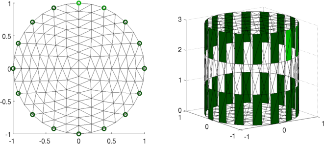
Figure: output image showing 2D and 3D EIT finite element models. Electrodes are shown in green. Electrode #1 is light green.

Create a simple 3D fwd_model structure

% Simulate EIT data
% $Id: tutorial010b.m 3273 2012-06-30 18:00:35Z aadler $

sim_img= mk_image(imdl_3d.fwd_model,1);

% set voltage and current stimulation patterns
stim =  mk_stim_patterns(16,2,[0,1],[0,1],{},1);
sim_img.fwd_model.stimulation = stim;

% set homogeneous conductivity and simulate
homg_data=fwd_solve( sim_img );

% set inhomogeneous conductivity and simulate
sim_img.elem_data([390,391,393,396,402,478,479,480,484,486, ...
                   664,665,666,667,668,670,671,672,676,677, ...
                   678,755,760,761])= 1.15;
sim_img.elem_data([318,319,321,324,330,439,440,441,445,447, ...
                   592,593,594,595,596,598,599,600,604,605, ...
                   606,716,721,722])= 0.8;
inh_data=fwd_solve( sim_img );

clf;subplot(211);

xax= 1:length(homg_data.meas);
hh= plotyy(xax,[homg_data.meas, inh_data.meas], ...
           xax, homg_data.meas- inh_data.meas );

set(hh,'Xlim',[1,max(xax)]);
print_convert('tutorial010b.png','-density 75');

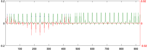
Figure: Simulated voltages from 3D EIT mesh. Right axis (left) shows the difference signal due to an inhomogeneity.

Reconstruct images

% Reconstruct images
% $Id: tutorial010c.m 2157 2010-04-04 11:22:54Z aadler $

subplot(131)
show_fem(sim_img);

%Add 20dB SNR noise to data
noise_level= std(inh_data.meas - homg_data.meas)/10^(20/20);
inh_data.meas = inh_data.meas + noise_level* ...
                randn(size(inh_data.meas));

%reconstruct 
rec_img= inv_solve(imdl_3d, homg_data, inh_data);

% Show reconstruction as a 3D mesh
subplot(132)
show_fem(rec_img)

subplot(133)
rec_img.calc_colours.npoints = 128;
show_slices(rec_img,[inf,inf,2.0,1,1; ...
                     inf,inf,1.0,1,2]);

print_convert('tutorial010c.png', '-density 100', 0.5);

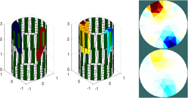
Figure: Left: Simulation image; Middle: Reconstructed image (as mesh); Right: Reconstructed image slices at z=1.0 and z=2.0.