EIDORS: Electrical Impedance Tomography and Diffuse Optical Tomography Reconstruction Software

Hosted by

Solving onto Nodes vs Elements

Solving onto Nodes vs Elements

% Simulate Target $Id: nodal_solve01.m 2157 2010-04-04 11:22:54Z aadler $

imdl= mk_common_model('d2d1c',16);
img= mk_image(imdl);

vh = fwd_solve(img); %Homogeneous
select_fcn = inline('(x-0.2).^2+(y-0.5).^2<0.1^2','x','y','z');
img.elem_data = 1 + elem_select(img.fwd_model, select_fcn);
vi = fwd_solve(img); %Homogeneous

subplot(221);
show_fem(img);
print_convert nodal_solve01a.png

plot([vh.meas, vi.meas]); axis tight
print_convert nodal_solve01b.png

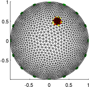
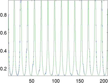
Figure: Simulation mesh (left)) and simulated voltages (right)

Reconstructing onto elements

% Element Solvers Target $Id: nodal_solve02.m 4839 2015-03-30 07:44:50Z aadler $

% Coarse model
imdl1= mk_common_model('a2c0',16);
imdl1.RtR_prior = @prior_laplace;
imdl1.hyperparameter.value = 0.1;

img1 = inv_solve(imdl1, vh, vi);
show_fem(img1);
print_convert nodal_solve02a.png

% Fine model
imdl2= mk_common_model('c2c0',16);
imdl2.RtR_prior = @prior_laplace;
imdl2.hyperparameter.value = 0.1;

img2 = inv_solve(imdl2, vh, vi);
show_fem(img2);
print_convert nodal_solve02b.png

Reconstructing onto nodes

% Element Solvers Target $Id: nodal_solve03.m 4839 2015-03-30 07:44:50Z aadler $

% Coarse model
imdl1= mk_common_model('a2c0',16);
imdl1.solve = @nodal_solve;
imdl1.RtR_prior = @prior_laplace;
imdl1.hyperparameter.value = 0.1;

img1 = inv_solve(imdl1, vh, vi);
show_fem(img1);
print_convert nodal_solve03a.png

% Fine model
imdl2= mk_common_model('c2c0',16);
imdl2.solve = @nodal_solve;
imdl2.RtR_prior = @prior_laplace;
imdl2.hyperparameter.value = 0.1;

img2 = inv_solve(imdl2, vh, vi);
show_fem(img2);
print_convert nodal_solve03b.png

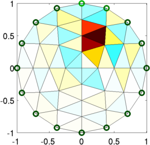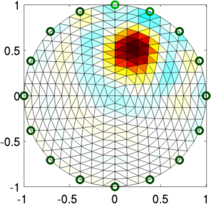
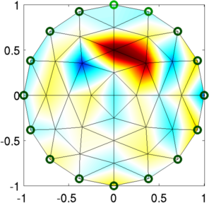
Figure: Reconstructed conductivity reconstructed to elements (top) and nodes (bottom)