EIDORS: Electrical Impedance Tomography and Diffuse Optical Tomography Reconstruction Software

Hosted by

EIDORS fwd_models

Creating an FEM and solving the forward problem

% Forward solvers $Id: forward_solvers01.m 3790 2013-04-04 15:41:27Z aadler $

% 2D Model
imdl= mk_common_model('d2d1c',19);

% Create an homogeneous image
img_1 = mk_image(imdl);
h1= subplot(221);
show_fem(img_1);

% Add a circular object at 0.2, 0.5
% Calculate element membership in object
img_2 = img_1;
select_fcn = inline('(x-0.2).^2+(y-0.5).^2<0.1^2','x','y','z');
img_2.elem_data = 1 + elem_select(img_2.fwd_model, select_fcn);

h2= subplot(222);
show_fem(img_2);

img_2.calc_colours.cb_shrink_move = [.3,.8,-0.02];
common_colourbar([h1,h2],img_2);

print_convert forward_solvers01a.png

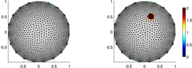
Figure: A 2D finite element model (left) and an conductivity contrasting inclusion (right)

% Forward solvers $Id: forward_solvers02.m 3790 2013-04-04 15:41:27Z aadler $

% Calculate a stimulation pattern
stim = mk_stim_patterns(19,1,[0,1],[0,1],{},1);

% Solve all voltage patterns
img_2.fwd_model.stimulation = stim;
img_2.fwd_solve.get_all_meas = 1;
vh = fwd_solve(img_2);

% Show first stim pattern
h1= subplot(221);
img_v = rmfield(img_2, 'elem_data');
img_v.node_data = vh.volt(:,1);
show_fem(img_v);

% Show 7th stim pattern
h2= subplot(222);
img_v = rmfield(img_2, 'elem_data');
img_v.node_data = vh.volt(:,7);
show_fem(img_v);

img_v.calc_colours.cb_shrink_move = [0.3,0.8,-0.02];
common_colourbar([h1,h2],img_v);
print_convert forward_solvers02a.png

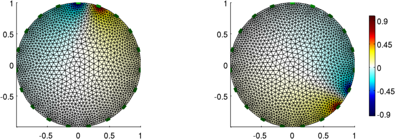
Figure: The voltage pattern from adjacent stimulation

% Forward solvers $Id: forward_solvers03.m 3790 2013-04-04 15:41:27Z aadler $

% Calculate a stimulation pattern
stim = mk_stim_patterns(19,1,[0,9],[0,1],{},1);

% Solve all voltage patterns
img_2.fwd_model.stimulation = stim;
img_2.fwd_solve.get_all_meas = 1;
vh = fwd_solve(img_2);

% Show first stim pattern
h1= subplot(221);
img_v = rmfield(img_2, 'elem_data');
img_v.node_data = vh.volt(:,1);
show_fem(img_v);

% Show 7th stim pattern
h2= subplot(222);
img_v = rmfield(img_2, 'elem_data');
img_v.node_data = vh.volt(:,7);
show_fem(img_v);

img_v.calc_colours.cb_shrink_move = [0.3,0.8,-0.02];
common_colourbar([h1,h2],img_v);

print_convert forward_solvers03a.png

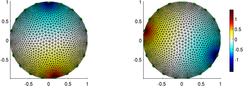
Figure: The voltage pattern from opposite (nearly) stimulation

% Forward solvers $Id: forward_solvers04.m 4062 2013-05-24 19:28:18Z bgrychtol $

% Calculate a stimulation pattern
stim = mk_stim_patterns(19,1,[0,1],[0,1],{},1);

% Solve all voltage patterns
img_1.fwd_model.stimulation = stim;
img_1.fwd_solve.get_all_meas = 1;
vh1= fwd_solve(img_1);

img_2.fwd_model.stimulation = stim;
img_2.fwd_solve.get_all_meas = 1;
vh2= fwd_solve(img_2);

img_v = rmfield(img_2, 'elem_data');

% Show homoeneous image
h1= subplot(231);
img_v.node_data = vh1.volt(:,1);
show_fem(img_v); axis equal

% Show inhomoeneous image
h2= subplot(232);
img_v.node_data = vh2.volt(:,1);
show_fem(img_v); axis equal

% Show difference image
h3= subplot(233);
img_v.node_data = vh1.volt(:,1) - vh2.volt(:,1);
show_fem(img_v); axis equal

img_v.calc_colours.cb_shrink_move = [0.3,0.8,-0.05];
common_colourbar([h1,h2,h3],img_v);

print_convert forward_solvers04a.png

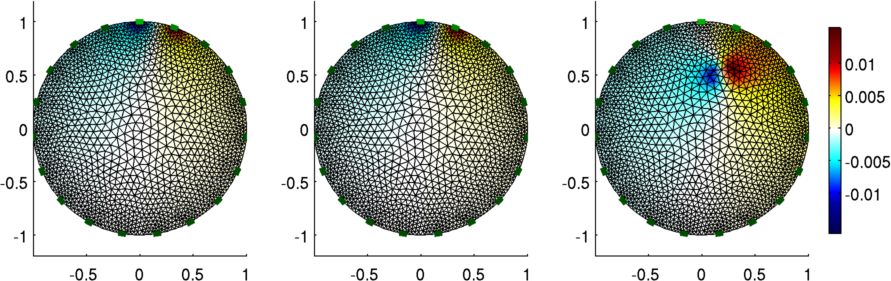
Figure: The voltage pattern from a change in conductivity

% Forward solvers $Id: forward_solvers05.m 3874 2013-04-17 19:32:11Z bgrychtol $


% Solve all voltage patterns
img_2.fwd_solve.get_all_meas = 1;
img_2.fwd_model.mdl_slice_mapper.npx = 64;
img_2.fwd_model.mdl_slice_mapper.npy = 64;

% Show [0-3] stim pattern
subplot(221);
stim = mk_stim_patterns(19,1,[0,3],[0,1],{},1);
img_2.fwd_model.stimulation = stim;
vh = fwd_solve(img_2);
show_current(img_2,vh.volt(:,1));
axis([-1,1,-1,1]); axis equal, axis tight

% Show [2-9] stim pattern
subplot(222);
stim = mk_stim_patterns(19,1,[0,7],[0,1],{},1);
img_2.fwd_model.stimulation = stim;
vh = fwd_solve(img_2);
show_current(img_2,vh.volt(:,3));
axis([-1,1,-1,1]); axis equal, axis tight

print_convert forward_solvers05a.png

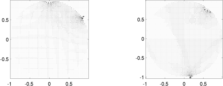
Figure: The current pattern for various stimulation patterns

Voltage and Current stimulation

Current (Dirichlet) boundary conditions

% Forward solvers $Id: forward_solvers06.m 5758 2018-05-19 20:37:04Z aadler $

% Simulation Image
imgs= mk_image(mk_common_model('d2d1c',21));
imgs.fwd_model.electrode = imgs.fwd_model.electrode([15:21,1:8]);
nel = num_elecs(imgs);
imgs.fwd_solve.get_all_meas = 1;

% Output Image
imgo = rmfield(imgs,'elem_data');
imgo.calc_colours.ref_level = 0;

% Regular "current" stimulation between electrodes 6 and 10
clear stim;
stim.stim_pattern = zeros(nel,1);
stim.stim_pattern([6,10]) =  [10,-10];
stim.meas_pattern = speye(nel);
imgs.fwd_model.stimulation = stim;

vh = fwd_solve( imgs ); imgo.node_data = vh.volt(:,1);

subplot(221); show_fem(imgo,[0,1]); axis off;

Voltage (Neumann) and Current (Dirichlet) boundary conditions

% Forward solvers $Id: forward_solvers07.m 5645 2017-09-10 20:33:02Z aadler $

% current stimulation between electrodes 6 and 10
stim.stim_pattern = zeros(nel,1);
stim.stim_pattern([6,10]) =  [10,-10];
% Voltage stimulation between electrodes 1,2 and 14,15
stim.volt_pattern = zeros(nel,1);
stim.volt_pattern([1,2,14,15]) =  [1,1,-1,-1]*5;
% Need to put NaN in the corresponding elements of stim_pattern
stim.stim_pattern([1,2,14,15]) =  NaN*ones(1,4);

imgs.fwd_model.stimulation = stim;
vh = fwd_solve( imgs ); imgo.node_data = vh.volt(:,1);

subplot(222); show_fem(imgo,[0,1]); axis off

print_convert forward_solvers07a.png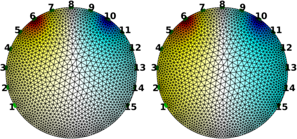

Figure: Left: Current specified on electrodes 6 and 10. Right: Voltage specified on electrodes 1,2,14,15 and current specified on electrodes 6 and 10.