| |
Ultrasound Image Processing
Analysis of Ultrasound images
Automatic analysis of medical images is somewhat controversial.
The advantages are clear: computer analysis is cheaper and
results will not vary for a given image. However, medical
images are highly variable. Algorithms are inherently
tuned to look for specific features, and are prone to
fail spectacularly when given unexpected input data.
My opinion is that the best current use of technology
is to assist trained technologists. It would attempt
to detect candidate features, but would require human
validation of all questionable decisions.
Example: Detection of Parameters for glaucoma measurement
Credit: Much of the analysis presented here is
from work by Pino Dicorato
Data analysed is from the paper:
Elucidating the mechanism of Occludable Angles
in patients with Pseudoexfoliation Syndrome
by
E.A. Ross
K.F. Damji
W.G. Hodge
A. Al-Ani
A.A. Al-Ghamdi
K. Shah
D. Chialant
This work performed by team at U. Ottawa Eye Institute.
Glaucoma is one of the leading causes of blindness in North-America
and around the world. In closed angled Glaucoma, high intraocular
pressure (fluid pressure in the eye) resulting from inadequate fluid
flow between the iris and the cornea causes damage and eventually death
of nerve fibres responsible for vision. One important technique to
assess patients at risk of glaucoma is to analyze ultrasound images of
the eye, for structural changes that reduce the outflow of fluids out
of the eye. Sequences of ultrasound images of the eye are analyzed
manually; anatomical feature locations are determined by a trained
technician, and relevant clinical parameters subsequently measured.
We discuss image processing techniques to automate the
location of clinically relevant features in ultrasound images of the
eye. We describe a feature detection algorithm to identify:
1) the location of the canal of Schlemm (drainage), 2) the location of
ciliary body, and 3) the angle formed between the iris and the cornea.
In this study, all image analysis was performed by a
trained technologist. We are interested in whether it
could be possible to automatically measure these parameters.
The expert measurements constitute the gold
standard against which computer estimates are
validated.
Technical Goal
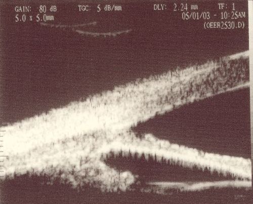
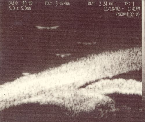
Measure the following parameters from images
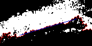
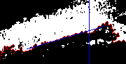
Example Images (Scanned from print-out):
| Open
| Closed
|
|
|
Image Processing
We illustrate steps involved to find Θ1 (the
apex of the angle is feature B)
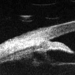
and the Scleral Spur (feature A). This illustrates some of the challenges
involved in such image processing. Examples are
based on this image
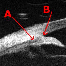
Ultra-sound image of Iris: Output from scanner to 3.5" disk.
Locate feature B
This feature is surprisingly hard to accurately obtain.
The following code samples are implemented in
octave, and
require the edge.m code from
octave.sf.net.
| Code
| Image
|
load and crop image region
im=imread('OCBX2614.jpg');
im= im(90:180,:);
imwrite('img-crop.jpg',im);

cmap= [0,0,0;1,1,1;0,0,.8;.8,0,0];
|
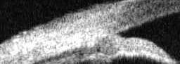
Image is cropped to show core region of interest
|
Sobel edge detecion
[im1, thresh] = edge( im, 'sobel');
%sobel:
% filt1= [1 2 1;0 0 0;-1 -2 -1];
% filt2= rot90( filt1 )
% combine= sqrt( filt1^2 + filt2^2 )
% Thresh= 23.1
imwrite('img-sobel.png',im1+1,cmap);
|
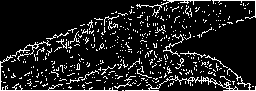
Problem is that there are holes in edge.
A fill will "pour" through holes
|
Lower Sobel edge threshol
im2 = edge( im, 'sobel', 10);
% Set threshold lower to get more edge
imwrite('img-sobel2.png',im2+1, cmap);
|
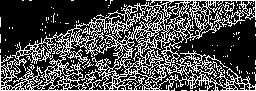
The edge is still unstable and we have artefacts
in the black region
|
Flood fill region of interest
bw= bwfill(im2, 45, 256,4);
% use 4 connected bw fill
fill= 2*bw - im2 + 1;
imwrite('img-s2fill.png',fill, cmap);
|
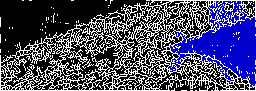
Note that the fill region (blue) penetrates
into the tissue region
|
Use Advanced Edge Detection (Canny type)
% Do Sobel edge detection to generate an image at
%  a high (HT) and low threshold (LT)
% Edge extend all edges in the LT image by several
%  pixels, in vertical, horizontal, and 45° dirns.
%  Combine these into edge extended (EE) image
% Dilate the EE image by 1 step
% Select all EE features that are connected to
%  features in the HT image
[im3, thresh] = edge( im, 'andy');
imwrite('img-andy.png',im3+1,cmap);
|

This works fairly well, but there
is some edge blurring.
|
Flood fill region of interest
bw= bwfill(im3, 45, 256,4);
fill= 2*bw - im3 + 1;
imwrite('img-a-fill.png',fill, cmap);
|

Now, we need to fit a triangle to this shape
|
Find top and bottom edge
im4= fill==3; % left-most filled point
leftpt= find( any(im4) )(1);
im5= im4( :, leftpt:size(im4,2) );
bw= bwfill(im5, 1, 1,4);
fill= im5 + bw + 1;
imwrite('img-fill2.png',fill, cmap);
|

Three regions are defined
|
Detect Edges
mask= [0,1,0;1,1,1;0,1,0]/5;
edge1= (conv2(fill==2,mask,'same')>0).*im5;
edge2= (conv2(fill==1,mask,'same')>0).*im5;
fill= 2*edge1 +1; fill(find(edge2))= 4;
imwrite('img-edge2.png',fill, cmap);
|

Red and blue lines mark the boundaries
|
Extract fit from lines
function [fit,idx]= imagefit( img, poly_degree )
   pt= find( img > 0 ) - 1; % we want 0 base index
   x= floor( pt / size(img,1) );
   y=   rem( pt , size(img,1) );
   fit = polyfit(x,y, poly_degree);
   yfit= polyval( fit, x);
   idx=  1+ round(x*size(img,1) + yfit);
endfunction

[fit,idx1]= imagefit( edge1,1);
[fit,idx2]= imagefit( edge2,1);

fill= im5+1; fill(idx1)= 3; fill(idx2)= 4;
imwrite('img-edge3.png',fill, cmap);
|

This doesn't work. We must force lines to meet at point B.
|
Extract fit. Lines must meet at centre, and only use
initial portion of section
function [fit,idx]= imagefit( img, uselim)
   pt= find( img(:,1:uselim) > 0 ) - 1;
   x= floor( pt / size(img,1) );
   y=   rem( pt , size(img,1) );
   ymean=  mean( find (img(:,1)) - 1);
   fit = [x\(y-ymean); 0]; % slope is x\y, intercept is 0
   yfit= polyval( fit, x) + ymean;
   idx=  1+ round(x*size(img,1) + yfit);
endfunction

[fit,idx1]= imagefit( edge1, 60);
[fit,idx2]= imagefit( edge2, 60);

fill= im5+1; fill(idx1)= 3; fill(idx2)= 4;
imwrite('img-edge4.png',fill, cmap);
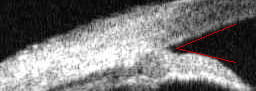
|

The point position and angle can now be determined
|
Global Picture
im(idx1+leftpt*size(im,1))=256;
im(idx2+leftpt*size(im,1))=256;
cmap2= [gray(256); [.8,0,0]];
imwrite('img-featb.png',im+1, cmap2);
|
Note that feature B is still not accurately
estimated.
Improvements are left as an
excercise for the reader 8-)
|
Locate feature A
This feature is difficult for many reasons.
Most importantly, ultrasound has intrinsically very low
SNR, due to Rayleigh scattering.
This means we cannot easily use contrast for
discrimination of regions in such tissue.
Some code to illustrate the effect of
Rayleigh scattering is
here.
| Code
| Image
|
load and crop image region
im=imread('OCBX2614.jpg');
im= im(110:200,:);
imwrite('img-crop2.jpg',im);

cmap2= [gray(256); [.8,0,0];[0,0,.8]];
|
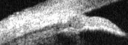
Image is cropped to show core region of interest
|
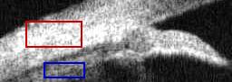
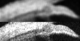
Select tissue regions
fill= im;
fill( 24:53, 29:91 ) = 256;
fill( 26:51, 31:89 ) = im( 26:51, 31:89 );
fill( 70:87, 49:94 ) = 257;
fill( 72:85, 51:92 ) = im( 72:85, 51:92 );
imwrite('img-region.jpg',fill+1,cmap2);
|
|
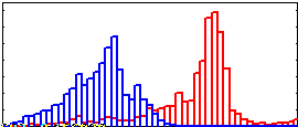
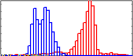
View Histograms
r1= im( 24:53, 29:91 );
hist( r1(:), 0:5:255, 1);
hold on
r2= im( 70:87, 49:94 );
hist( r2(:), 0:5:255, 1);
|
Horiz axis is 0 to 255. Regions are faily distinct.
|
Threshold at crossover point
imt= im>170;
imwrite('img-t1.png',imt+1,cmap);
|
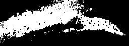
Threshold works quite well in centre of
region, but not well in bottom left
|
Crop and fill from bottom
imt2= imt(:,1:180);
bw= bwfill(imt2, size(imt2,1), 1, 4);
fill= 2*bw - imt2 + 1;
imwrite('img-t2.png',fill,cmap);
|
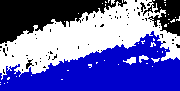
blue region has "holes"
|
Fill holes in blue region
bw = fill==3;
bw2= bwfill(bw, 'holes', 4);
imwrite('img-t3.png',bw2 + 1,cmap);
|

|
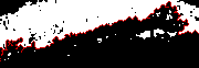
Find edge
mask= [0,1,0;1,1,1;0,1,0]/5;
edge= (conv2(bw2,mask,'same')>0).*(1-bw2);
fill= imt2 +1; fill(find(edge))= 4;
imwrite('img-edget.png',fill(30:size(fill,1),:), cmap);
|
|
Fit line to straight segment
function [fit,idx]= imagefit( img, poly_degree )
   pt= find( img > 0 ) - 1; % we want 0 base index
   x= floor( pt / size(img,1) );
   y=   rem( pt , size(img,1) );
   fit = polyfit(x,y, poly_degree);
   yfit= polyval( fit, x);
   idx=  1+ round(x*size(img,1) + yfit);
endfunction

[fit,idx1]= imagefit( edge(:,38:149),1);
fill2= fill;
fill2(idx1 + size(fill,1)*38)= 3;
imwrite('img-edgef.png',fill2, cmap);
|
|
Find edge point maximum depth below line
for i=39:149
   edge_y(i)= mean(find(fill(:,i)==4));
   line_y(i)= mean(find(fill2(:,i)==3));
end
dif=  edge_y - line_y;
ptx= mean( find( dif == max(dif) ) );
fill2(:,round(ptx))= 3;
imwrite('img-edgep.png',fill2, cmap);
|
|
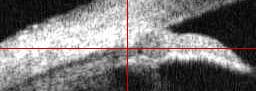
On the original image this gives
pty= mean(find(fill(:,round(ptx))==4));
fill= im;
fill( :, round(ptx) ) = 256;
fill( round(pty), : ) = 256;
imwrite('img-ptA.jpg',fill+1,cmap2);
|
|
While this works, for this particular image, this processing
is fairly unreliable, because:
- The threshold value needs to be accurately chosen
- The horizontal limits for the line fit need to be
accurately chosen
In the following section, we focus on a technique to
better separate the regions to find an appropriate threshold.
The essense of these techniques is to use texture analysis.
NOTE: This material is for explanation of
the concepts of texture analysis. Correct implementation
of these ideas uses techniques such as
Markov random fields.
| Code
| Image
|
Analyse region autocorrelations
sz= 8; sz2= 2*sz+1;

xc1= xcorr2(r1, 'unbiased');
xctr= ceil(size(xc1,2)/2);
yctr= ceil(size(xc1,1)/2);
xc1=xc1( yctr+(-sz:sz), xctr+(-sz:sz));
xc1=xc1/sum(xc1(:));

xc2= xcorr2(r2, 'unbiased');
xctr= ceil(size(xc2,2)/2);
yctr= ceil(size(xc2,1)/2);
xc2=xc2( yctr+(-sz:sz), xctr+(-sz:sz));
xc2=xc2/sum(xc2(:));

minfill= min([xc1(:);xc2(:)]);
fill= [xc1-minfill, zeros(sz2,2), xc2-minfill];
imwrite('img-xcorr.jpg',255*fill/max(fill(:)));
|

Xcorr of R1 on left and R2 on right
R1 is more spatially uniform than R2
|
Develop a "sample" of regions
sz2= 2*4+1;

f1e= interpft( fft2(r1), 2*sz2, 2*sz2 );
i1e= real(ifft2(f1e)); i1e=i1e(1:sz2, 1:sz2);
imwrite('img-r1e.jpg',i1e);

f2e= interpft( fft2(r2), 2*sz2, 2*sz2 );
i2e= real(ifft2(f2e)); i2e=i2e(1:sz2, 1:sz2);
imwrite('img-r2e.jpg',i2e);
|


|
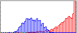
Original histogram of regions
|
|
Selectively Enhance with region 1
r1h= xcorr2(r1,i1e,'unbiased')(:);
r2h= xcorr2(r2,i1e,'unbiased')(:);
scale= 255/max([r1h;r2h]);
hold off; hist(scale*r1h, 0:5:250, 1);
hold on; axis ([0, 250, 0, .15]);
hist(scale*r2h, 0:5:250, 1);
|
Region 2 now overlaps Region 1
|
Selectively Enhance with region 2
r1h= xcorr2(r1,i2e,'unbiased')(:);
r2h= xcorr2(r2,i2e,'unbiased')(:);
scale= 255/max([r1h;r2h]);
hold off; hist(scale*r1h, 0:5:250, 1);
hold on; axis ([0, 250, 0, .15]);
hist(scale*r2h, 0:5:250, 1);
|
Greater separation between regions
|
Enhance image with region 2
ime2= xcorr2(im, i2e, 'unbiased');
ime2= ime2-min(ime2(:));
ime2= 255*ime2/max(ime2(:));
ime2crop= ime2(20:size(ime2,1)-10,5:size(ime2,2)-4);
fill= [ ime2crop; im(25:size(im,1)-6,:)];
imwrite('img-e2.jpg',fill);
|
Greater separation between regions
|
Last Updated:
$Date: 2004-04-12 09:48:56 -0400 (Mon, 12 Apr 2004) $
|