This page gives a brief tour of MProbe version 3.0, complete with screen shots. For best viewing, you should maximize your browser since the screen shots are full size.
Note throughout that MProbe is specifically designed to operate on functions of many variables. This is especially true of the methods for estimating the shape (convex? concave? both? linear? etc.) of nonlinear functions having too many variables to simply plot and analyze by eye.
Before beginning with MProbe, let's first take a brief look at a simple AMPL model file: test6.txt . The syntax in this simple example is straightforward.
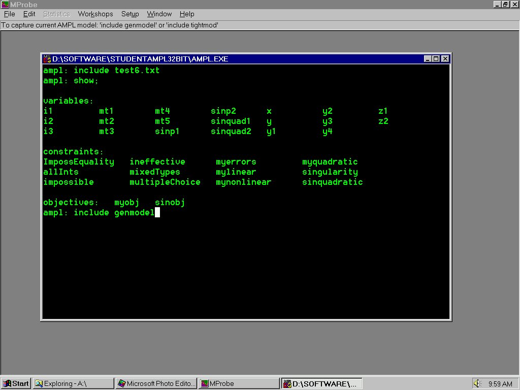
Slide 1 shows MProbe after start-up, and after AMPL has been started (by choosing File|Start AMPL from the menu. Three AMPL commands show in the AMPL window:
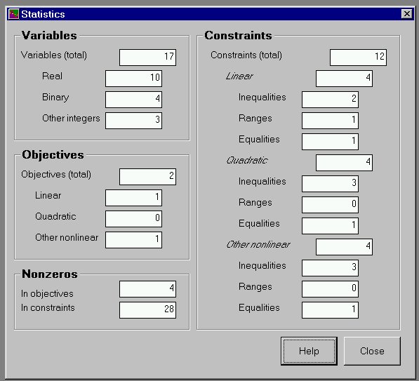
Slide 2 shows the Statistics window which appears after the AMPL model is read by MProbe. The Statistics window can be recalled anytime from the menu.
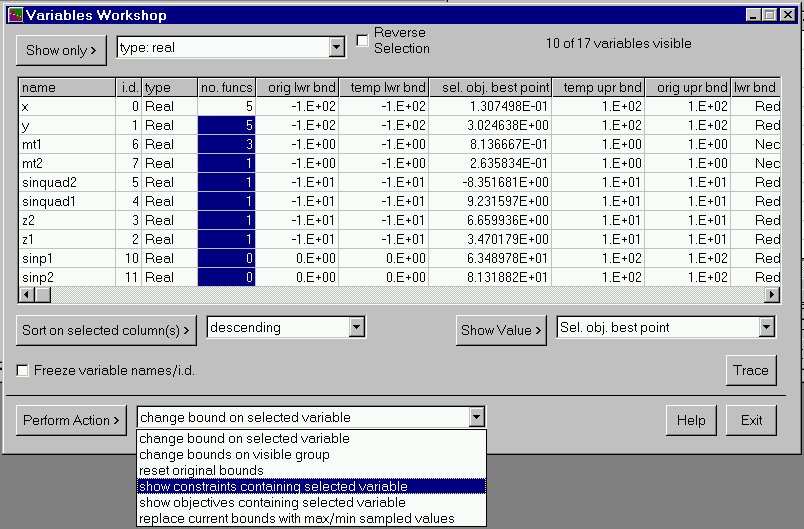
Slide 3 shows the Variables Workshop window. The spreadsheet-like grid shows information about the variables: their names, types, number of functions they appear in, and original and temporary upper and lower bounds. You can select a subset of variables to view in the grid by choosing a criterion from the Show Only list (only the real-valued variables are shown in this example). You can sort the variables by selecting columns on which to sort, and pressing the Sort on selected column(s) button (the variables in this example are sorted according to the number of functions they appear in). A set of actions, such as showing all the constraints that contain a selected variable, is also available via the Perform Action button. For example, you could find a useful ordering for the variables in a MIP by viewing only the integer and binary variables, and then sorting them in descending order according to the number of functions they appear in.
The example also shows the best point for the currently selected variable (i.e. sampled point having maximum or minimum value of the objective, as appropriate), as found during a complete analysis of the model.
As in all of the grid displays in MProbe, the column widths are resizable. You can also expand the window to see more of the display, or you can select the checkbox to freeze the variable identification so that it is always visible onscreen.
It is important to understand that MProbe derives a lot of information by sampling the variable space. It scatters random line segments of random length throughout the space defined by the temporary bounds on the variables. Comparing the function value at a point with a value interpolated from the two random line endpoints indicates whether the function is concave or convex at that point. This information can be collected in a histogram, as can other information gleaned from the sampling, such as data on function values, constraint effectiveness, etc.
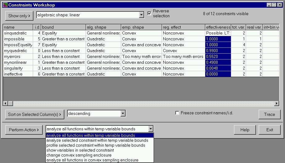
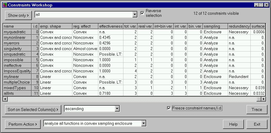
Slide 4 shows the Constraints Workshop, which summarizes the information about the constraints: name, type of relationship, algebraic shape, empirical shape in the space defined by the temporary bounds, the effect the constraint has on the constrained region, the estimated effectiveness (fraction of the variable space removed by the constraint), and counts of the types of variables in the constraint. There is a long list of ways to select constraints for viewing using the Show Only list and button. In the slide, only constraints whose algebraic shape is nonlinear are shown (this is 8 of 12 of the constraints in the model, as shown in the upper left).
Note that equality constraints such as sinquadratic do not have a simple effectiveness; instead there is an estimation as to whether or not it is possible to satisfy the equality at some point in the current variable space. Note also that an empirical shape of too many math errors is recorded if there are errors in evaluating a function (e.g. a divide by zero or other problem). As for the Variables Workshop, the grid display can be sorted on user-selected columns. In the slide, the constraints are sorted in decreasing order of effectiveness. This can be useful in constraint logic programs: the most effective constraints should be put first in the constraint list to encourage the development of small search trees.
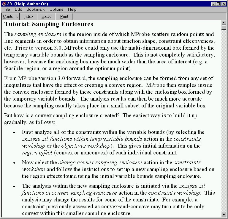
The slide also shows the list of actions that can be performed. The last two actions refer to "sampling enclosures". This is a new feature in version 3.0. Instead of sampling inside the multidimensional "box" formed by the variable bounds, you can sample inside any convex enclosure formed by inequalities in the model. The results of such an analysis are shown in slide 5. The constraints which form the enclosure are analyzed to estimate whether they are redundant or necessary. If an enclosure constraint is necessary, then the fraction of the total "surface" of the enclosure that the constraint comprises is also estimated.
Constraints that do not form the sampling enclosure are analyzed within the enclosure. This provides a much more accurate analysis of the relevant shape and effectiveness data. For example, a constraint estimated to have a "convex and concave" shape within the larger enclosure formed by the variable bounds, may well be found to have a convex or even linear shape when examined inside a tighter convex enclosure. Sampling enclosures are found by first sampling within the variable bounds, then using the empirical shape information to build up a tighter convex sampling enclosure. Information is also kept on the best values of the objective function encountered along the way.
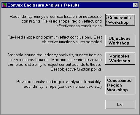
Slide 6 shows that sampling within the convex enclosure provides a broad range of information not previously available.
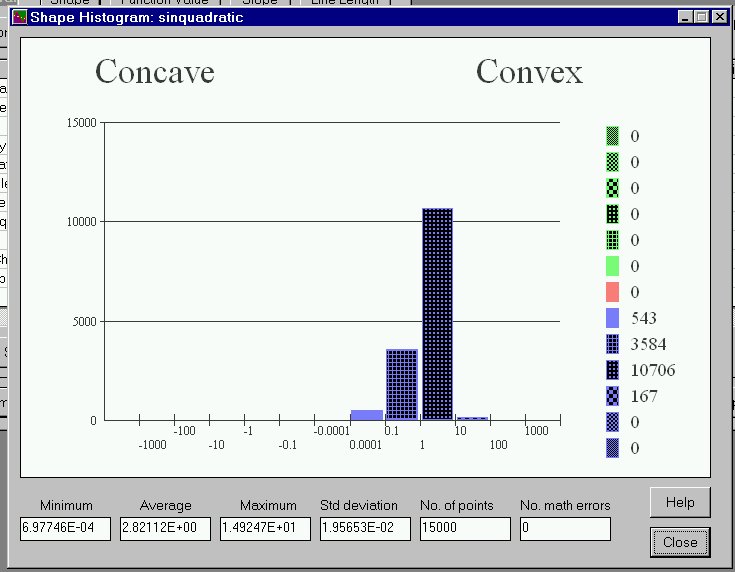
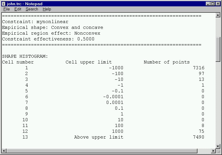
When functions (constraints or objectives) are analyzed individually, then detailed histograms of the shape analysis are returned. Slide 7 shows the shape histogram returned when the constraint sinquadratic is analyzed. This constraint is convex, within the tolerances specified by the user. It is not particulary deeply convex as shown by the average and maximum values in the histogram. Histograms are also generated for the function values, "slope" (change in function value between the line segment endpoints divided by the line length), and the length of the test lines.
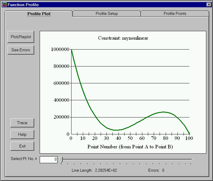
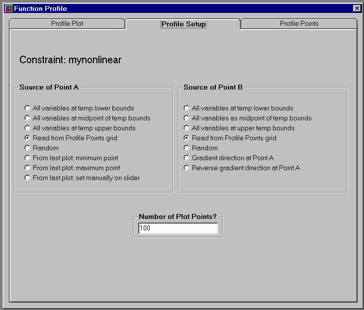
An interestying facility launched from the Constraints Workshop or the Objectives Workshop is "Function Profiling". This is a plot of the values of a function from some Point A in n-space to some other Point B in n-space along a straight line connecting those two points. The mynonlinear constraint is profiled in Slide 8 between two points in the 2-space that it occupies. It is certainly nonlinear by inspection! Slide 9 shows that there are numerous ways to set up a profile plot, including randomly, between user-specified points, or along the gradient direction. The actual values of Points A and B, and the facilities to modify them, are on the third tab, "Profile Points".
Function Profiling is useful when, for example, your solver is stuck at some Point A, but a better Point B is known to exist. The function profile between those two points in n-space might show an unexpected hill.
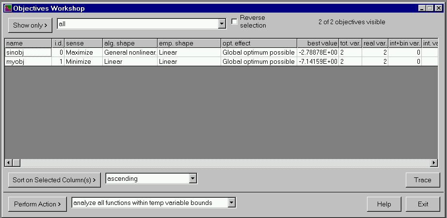
Slide 10 shows the Objectives Workshop. The sinobj objective function is linear with a small superimposed sinusoid, but when sampled inside the convex sampling enclosure, turns out to have a linear empirical shape! This means that the "optimum effect" is "global optimum possible". The best value of each objective found during sampling is also shown. An action available via the list in the lower left will display the point corresponding to the best value of the objective function.
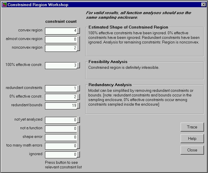
Slide 11 shows the Constrained Region Workshop after an analysis within a convex sampling enclosure. Three major analyses are performed: overall shape of the constrained region (convex? nonconvex?), feasibility, and redundancy. The numbers of constraints in various categories are shown, and the button next to each constraint count will take you to the Constraints Workshop loaded with the relevant constraints. Note that the "constrained region" is not the same as the "feasible region". The feasible region, if one exists, is a subset of the constrained region. It is important to know about the larger constrained region, as this affects the behaviour of phase-1 procedures, for example.
Slide 12 shows the Trace File. This is a user-controlled text file record of the session that can be viewed, annotated, saved, printed, etc. Relevant information is written to the trace file either automatically, or via the Trace button on most windows.
And finally, Slide 13 shows that MProbe comes with a complete help system. A number of tutorials are included to get you up to speed quickly.
Back to the MProbe home page.
Latest revision: November 16, 2001.