
|
|
Carleton
|
ELG 7173 - Human Visual SystemBlock Diagram Model of Monochrome vision Figure 1: Block Diagram Model of Monochrome vision The model of figure 1 considers four stages of vision:
Deficiencies of this model:
Mach BandsMach bands are adjacent vertical stripes of increasing grey level.They may be created using the following Matlab code: colours= 256; levels = 10; hsize= 250; vsize= 100; colormap( gray(colours) ); hline= ceil( linspace( 1, levels+1, 250) )* colours/(levels + 2); image( ones( vsize,1 ) *hline);  Figure 2: Mach Band Image In order to model the spatial frequency at which lateral inhibition operates, we construct in image with several different levels of low pass filter. In order to do this, we use the following code
colours= 256;
levels = 10;
hsize= 250;
vsize= 8;
colormap( gray(colours) );
hline= ceil( linspace( 1, levels+1, 250) )* colours/(levels + 2);
pad_hline= [min(hline)*ones(1,hsize), ...
            hline, ...
            max(hline)*ones(1,hsize) ]; % smooth padding each side
for kernel_width= [ 0.01, .025, .05, .1:.1:.5]
    conv_kernel= ones(1, hsize/levels*kernel_width );
    conv_kernel= conv_kernel / sum( conv_kernel );
    ft_hline= conv2( pad_hline, conv_kernel, 'same');
    ft_hline= ft_hline( hsize+(1:hsize) );
    img= ones( vsize,1 ) * ft_hline;
    jpgwrite( sprintf('mach-band-filter-%0.3f.jpg',kernel_width), img );
end
Each image has a different convolution kernel, and therefore, a
different spatial low pass filter.
Note that this effect will vary significantly as you move
toward and away from the screen.
Frequency dependence of contrast sensitivityNow we would like to understand the frequency dependence of contrast sensitivityThe following code plots an image contasts at different spatial frequencies. hsize= 500; vsize= 400; spread=8; freq= linspace(.01^(1/spread),1, hsize).^spread * .3; % freq is 1/2/pi * dw / dx w= 2*pi*cumsum( freq ); hline= sin(w); vline= linspace(0,1,vsize).^3; im= vline'*hline; imagesc(im); 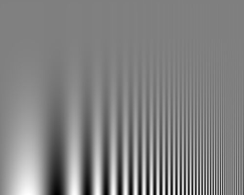 Figure 4: Image of contrasts at various spatial frequencies Note that contrasts are more visible at certain spatial frequencies than others. Thus you should be able to see the contrast further up the line in the center part of the figure. NOTE: Your monitor must be configure to use 24 or 32 bit colour for the effect to be visible. Unfortunately, occasionally, I've noticed windows will claim to be in 24 bit colour but actually will display in less colours. Last Updated: $Date: 2003-08-01 23:07:45 -0400 (Fri, 01 Aug 2003) $ |


