| |
ELG 7173 - Assignment #2
- Nuclear Medical Imaging

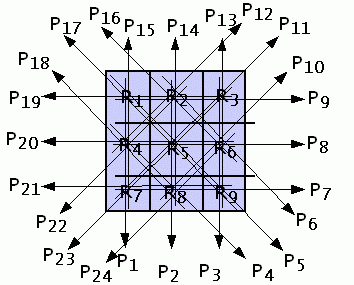
Figure Q1: Diagram for question 1.
Figure Q1 shows the nuclear medical imaging
projection data acquired from a simple
object with nine regions R1 to R9,
and twenty four data projections,
P1 to P24.
The projection calculations are indicated by the arrows;
for example, P1 is calculated as
the photons received along the axis through
R1, R4 and R7.
Assume each region is 2 cm wide, no matter whether it
is traversed from the edge or sides.
Consider a SPECT Imaging model, where
region R5 contains a radioisotope, and is
emitting 1000 γ particles along each of the eight projection
lines
per unit time. All other regions have no activity.
Each projection is the number of γ's received
per unit time.
- Initially, consider all regions to have
zero attenuation.
Calculate the value of all projections
P1 to P24, for this condition.
-
Using simple (ie. unfiltered) backprojection, calculate
the reconstructed activity in each region,
for these projection data.
- Now, consider regions
R1, R2, and R3 to
have attenuation of 0.2 cm-1,
regions
R4, R6,
R7, R8, and R9 to
have attenuation of 0.1 cm-1.
Calculate the value of all projections
P1 to P24, for this condition.
-
Using simple (ie. unfiltered) backprojection, calculate
the reconstructed activity in each region,
for these projection data.
-
Comment briefly on the impact of attenuation
on Nuclear Medical Images
- Nuclear Medical Imaging
-
In class we have discussed three kinds of collimation:
1) Pinhole collimation
2) Electronic collimation
3) Parallel hole collimation.
Discuss each collimation technology, describing
one medical imaging application.
-
Discuss two issues (of the three presented in class)
to be considered in the choice of isotopes
for nuclear medical imaging (max 100 words/answer).
-
A new detector technology is invented for PET which allows
the difference in timing of coincidence events to be measured
to an accuracy of 1 ns.
Describe how such information can be used to improve PET image
reconstruction.
Specifically, describe in general terms how backprojection
reconstruction could be modified to use this information.
-
Why is attenuation correction important for Nuclear Medical
image reconstruction?
In class we discussed three methods to estimate the data
necessary for attenuation correction.
Describe one method to estimate attenuation.
- MRI Fourier transform imaging

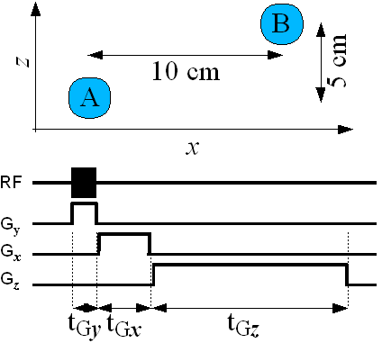
Figure Q2: Diagram for question 2.
Figure Q2 shows two contrasting regions, A and B, in an otherwise
empty space. The MRI z axis (frequency encoded)
and
x axis (phase encoded)
are shown. The timing diagram for the
pulse sequence (90°-FID) is also shown.
The magnetic field B0 is 1.5T. All gradient
field strengths are 1 Gauss/cm. The RF field strength
is 0.05 Gauss, and the shape of the RF pulse is
rectangular. Hydrogen is being imaged (γ=42.58 MHz/T)
-
What is the bandwidth of the RF receiver required
to image the field of view including A and B.
-
It is desired that the phase difference between A
and B be 180°.
Which timing parameter does
this contrain, and what is its value?
-
The RF pulse length is set to achieve the 90° rotation in
Nuclear Magnetic Field.
Which timing parameter does
this contrain, and what is its value?
- MRI Imaging Protocols
-
Consider the following MRI pulse sequences:
90°-FID and Spin-echo.
Explain, using graphs as necessary, how Spin-Echo
allows distinguishing tissues which differ in
T2 but not T1, while
90°-FID does not.
Two tissue regions (A and B) are being imaged with a Spin-Echo
pulse sequence, and have parameters
T1, T2, and ρ*
as follows:
| Tissue
| T1 (s)
| T2 (ms)
| ρ*
|
| A
| 1.0
| 80
| 50
|
| B
| 0.8
| 120
| 40
|
The MRI signal for Spin-Echo imaging is proporional to
ρ*
×
( 1 − exp(−TR / T1 ) )
×
exp (−TE / T2 )
-
Derive an expression for the conditions
(TR and TE) which maximizes
the contrast between regions A and B.
Note: you should be able to solve for one parameter.
The solution for the other parameter can be left as
a non-linear differential equation.
-
A particular MRI machine has settings of
TR of 1.0s, 1.5s and 2.0s
and settings of
TE of 100ms and 150ms.
Which settings should be chosen for maximum contrast
between tissues A and B?
- MRI Simulation (Bonus question)
The following Matlab function mri_signal
simulates an MRI RF signal output, for a given
image matrix img,
scale [pixels/cm],
x-Gradient [Gauss/cm],
y-Gradient [Gauss/cm],
main Magnetic field B0 [Tesla],
T2* T2star,
Simulation time Tlim [µs], and
Sample time Ts [µs].
function rf=mri_signal( img, scale , Gx, Gy, Ty, B0, T2star, Tlim, Ts)
% simulate rf signal for MRI pulse sequence
% rf=mri_signal( sig_params, scale , Gx, Gy, B0, T2star, Tlim, Ts)
% img [szY x szX] image of MRI signal (ie rho*(1-exp(-TR/T1)*exp(-TE/TR) for spin echo)
% scale       image scale (pixels/ cm)
% Gx          is x gradient (freq  encoding) in Gauss/cm
% Gy          is y gradient (phase encoding) in Gauss/cm
% Ty          is phase encoding time in microseconds
% B0          is magnetic field in Telsa
% T2star      T2* spin relaxation in microseconds
% Tlim        the recording time (in microseconds)
% Ts          RF signal sampling time resolution (microseconds)

Gx= Gx*1e-4; Gy= Gy*1e-4; %convert to Tesla
Gyromagenticratio = 42.6; %Mhz/Tesla

% Note this assumes a point phase source for each voxel,
% this introduces artefacts into the images
[szX, szY] = size( img );
phase= 2*pi*Ty*Gy*Gyromagenticratio*( -(szY-1)/2:(szY-1)/2 )*scale ;

imgX= exp( 1j*phase ) *img;
f_min= Gyromagenticratio*(B0 - Gx*(szX-1)/2*scale );
f_max= Gyromagenticratio*(B0 + Gx*(szX-1)/2*scale );
ft_img= interp1( linspace(f_min, f_max, szX ), imgX, ...
      0:1/Tlim:1/Ts, ... % size of FFT domain,
      'linear',0);   % freq is zero outsize domain

ft= [ ft_img, fliplr( conj(ft_img(2:end-1)) ) ];
rf= ifft(ft);
if std(imag(rf))>1e-10; error('something wrong with code'); end
time1= 1:Tlim/Ts;
rf=real(rf(time1)).*exp( -Ts*time1/T2star );
The following sample code allows reconstruction
of an MRI image based on multiple simulations
using this software.
spc=.05  ; rlim=1;
[x,y]= meshgrid(-rlim:spc:rlim,-rlim:spc:rlim);
plen= size(x,1);
img = .0*((x.^2 + y.^2) > rlim);
img( x >.45 & x<.65 & y>-.05 & y<.45) =1;
img( x >-.55 & x<-.25 & y>.45 & y<.65) =1;
scale=1;
T2star= 50;
B0= 0.5; % To increase B, decrease Ts;
G= 10;

Gyromagenticratio = 42.6; %Mhz/t
Ts= 0.01;
Tlim= 100;

szX= size(img,2);
max_f= Gyromagenticratio*(B0 + G*1e-4*(szX-1)/2*scale ) *Tlim/2;
min_f= Gyromagenticratio*(B0 - G*1e-4*(szX-1)/2*scale ) *Tlim/2;
freq_range= floor(min_f):ceil(max_f);
mri= [];
for Ty= you need to figure this out here
    rf = mri_signal(img, scale , G, G, Ty, B0, T2star, Tlim, Ts);
    ft= fft(rf);
    mri= [mri;ft(freq_range)];
end

fm= ifftshift(ifft(mri));imagesc(abs(fm)');
Question: Find an appropriate selection of time steps Ty
to reconstruct the image. Show your reconstructed image, and briefly
describe any defects in it, in terms of the simulation or reconstruction
software.
Last Updated:
$Date: 2007-02-02 14:12:04 -0500 (Fri, 02 Feb 2007) $
|


 Engineering
 SCE
SCE
 Faculty
 A. Adler
 Courses
 ELG7173
 Assignment 2