EIDORS: Electrical Impedance Tomography and Diffuse Optical Tomography Reconstruction Software

Hosted by

EIDORS fwd_models

Complete electrode model (CEM) convergence study using higher order finite elements methods (FEM)

• M G Crabb. EIT Reconstruction Algorithms for Respiratory Intensive Care. PhD Thesis, University of Manchester, 2014.
• M G Crabb. Convergence study of 2D forward problem of electrical impedance tomography with high-order finite elements. Inverse Problems in Science and Engineering, 2016.

Methods and Results

nmesh = 3; %greater or equal 4 for sensible rate estimates (depends on computer architec)

%Build a square CEM model
%Nodal coordinates and electrode nodes 
x=linspace(0,pi,6); 
y=linspace(0,pi,6);
[X,Y]=meshgrid(x,y); vtx=[X(:) Y(:)];
elec_nodes={[0 0],[0,pi]};
mdl=mk_fmdl_from_nodes(vtx,elec_nodes,0.02,'name');

%Electrode node indices and nodes on boundary not on elecs
mdl.electrode(1).nodes = [7,13];
mdl.electrode(2).nodes = [19,25];
bound_nodes_not_elecs = [1,2,3,4,5,6,12,18,24,30,31,32,33,34,35,36];
    
%Make image and add some fields
img=mk_image(mdl,1); %figure; show_fem(img);
stim = mk_stim_patterns(2,1,'{ad}','{ad}',{'meas_current'}, 1);
mdl.stimulation=stim; 
img.fwd_model.bound_nodes_not_elecs=bound_nodes_not_elecs;   
mdl.bound_nodes_not_elecs=bound_nodes_not_elecs;
img.fwd_model.stimulation=stim; img.fwd_solve.get_all_meas=1;  
mdl_init=mdl;


%Copy model, assign unit conductivity and plot
mdl_h1=mdl; img_h1=mk_image(mdl_h1,1);
figure; 
subplot(121); show_fem(img_h1); hold on;
plot(img_h1.fwd_model.nodes(bound_nodes_not_elecs,1),...
img_h1.fwd_model.nodes(bound_nodes_not_elecs,2),'r*');
xlab = xlabel('x'); set(xlab,'FontSize',14);
ylab = ylabel('y'); set(ylab,'FontSize',14);      

%Refine model
mdl_h2=h_refine_square_domain(mdl); img_h2=mk_image(mdl_h2,1);
subplot(122); show_fem(img_h2); hold on;
plot(img_h2.fwd_model.nodes(bound_nodes_not_elecs,1),...
img_h2.fwd_model.nodes(bound_nodes_not_elecs,2),'r*');
xlab = xlabel('x'); set(xlab,'FontSize',14);
ylab = ylabel('y'); set(ylab,'FontSize',14);      

print_convert error_rates_contact_impedance01a.png

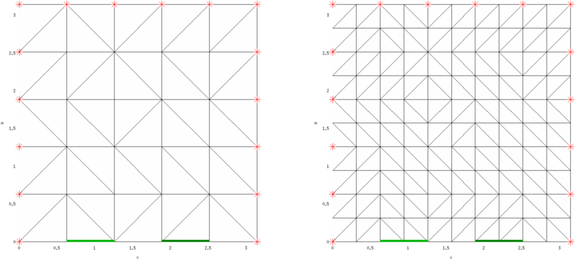
Figure: Initial 3D finite element model (left) and the same model after a single uniform h-refinement. The CEM electrodes (to drive voltage) are green lines and the (point) voltage measurement electrodes are red crosses.

%Loop over contact impedances
z_c=[0.00001,0.0001,0.001,0.01,0.1,1,10,100,1000];
for z_cj=1:length(z_c) % z_c=[0.1,1000];
%Reinitialise model and make image
mdl=mdl_init; img=mk_image(mdl,1);
mdl.electrode(1).z_contact = z_c(z_cj); 
img.fwd_model.electrode(1).z_contact=z_c(z_cj);
mdl.electrode(2).z_contact = z_c(z_cj); 
img.fwd_model.electrode(2).z_contact=z_c(z_cj);

%Solve forward problem with linear, quadratic, cubic and find H1-error
tic;
  fprintf(1,'H1 Lin');
  [lin_errL2(1,z_cj),lin_errH1(1,z_cj),lin_errH1tot(1,z_cj),lin_errI(1,z_cj), ...
   lin_errUS(1,z_cj),lin_errUM(1,z_cj),lin_errUSM(1,z_cj), ...
   lin_timing_solver(1,z_cj),lin_DOF(1,z_cj)]= calc_error_norms_for_square_domain(img,'tri3',1);
toc;
tic;
  fprintf(1,'H1 Quad');
  [quad_errL2(1,z_cj),quad_errH1(1,z_cj),quad_errH1tot(1,z_cj),quad_errI(1,z_cj), ...
  quad_errUS(1,z_cj),quad_errUM(1,z_cj),quad_errUSM(1,z_cj), ...
  quad_timing_solver(1,z_cj),quad_DOF(1,z_cj)]= calc_error_norms_for_square_domain(img,'tri6',1);
toc;
tic; fprintf(1,'H1 Cub'); 
	[cub_errL2(1,z_cj),cub_errH1(1,z_cj),cub_errH1tot(1,z_cj),...
	cub_errI(1,z_cj),cub_errUS(1,z_cj),cub_errUM(1,z_cj),cub_errUSM(1,z_cj),cub_timing_solver(1,z_cj),...
	cub_DOF(1,z_cj)]=calc_error_norms_for_square_domain(img,'tri10',1); toc;           

%Loop over different refinements
for ii=1:nmesh-1
    %Refine model uniformly and find errors with lin, quad, cubic                
    mdl=h_refine_square_domain(mdl);  img=mk_image(mdl,1);        
    tic; fprintf(1,'H1 Lin'); 
			[lin_errL2(ii+1,z_cj),lin_errH1(ii+1,z_cj),...
			lin_errH1semi(ii+1,z_cj),lin_errI(ii+1,z_cj),lin_errUS(ii+1,z_cj),lin_errUM(ii+1,z_cj),...
			lin_errUSM(ii+1,z_cj),lin_timing_solver(ii+1,z_cj),lin_DOF(ii+1,z_cj)]=...
			error_2D_squ_CEM(img,'tri3',0); toc;
    tic; fprintf(1,'H1 Quad'); 
			[quad_errL2(ii+1,z_cj),quad_errH1(ii+1,z_cj),...
			quad_errH1semi(ii+1,z_cj),quad_errI(ii+1,z_cj),quad_errUS(ii+1,z_cj),quad_errUM(ii+1,z_cj),...
			quad_errUSM(ii+1,z_cj),quad_timing_solver(ii+1,z_cj),quad_DOF(ii+1,z_cj)] = ...
			error_2D_squ_CEM(img,'tri6',0); toc;
    tic; fprintf(1,'H1 Cub'); 
			[cub_errL2(ii+1,z_cj),cub_errH1(ii+1,z_cj),cub_errH1semi(ii+1,z_cj),...
			cub_errI(ii+1,z_cj),cub_errUS(ii+1,z_cj),cub_errUM(ii+1,z_cj),cub_errUSM(ii+1,z_cj),...
			cub_timing_solver(ii+1,z_cj),cub_DOF(ii+1,z_cj)]=error_2D_squ_CEM(img,'tri10',0); toc;           
end

%Refine model uniformly and find errors with lin               
mdl=h_refine_square_domain(mdl);  img=mk_image(mdl,1);        
tic; fprintf(1,'H1 Lin'); 
	[lin_errL2(nmesh+1,z_cj),lin_errH1(nmesh+1,z_cj),...
	lin_errH1semi(nmesh+1,z_cj),lin_errI(nmesh+1,z_cj),lin_errUS(nmesh+1,z_cj),...
	lin_errUM(nmesh+1,z_cj),lin_errUSM(nmesh+1,z_cj),lin_timing_solver(nmesh+1,z_cj),...
	lin_DOF(ii+1,z_cj)]=error_2D_squ_CEM(img,'tri3',0); toc;       
end

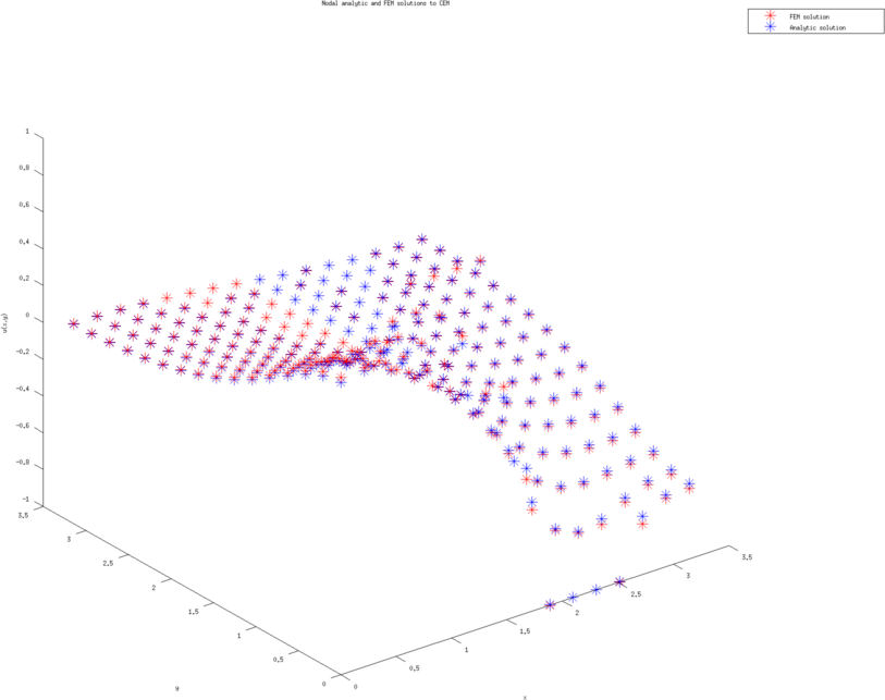
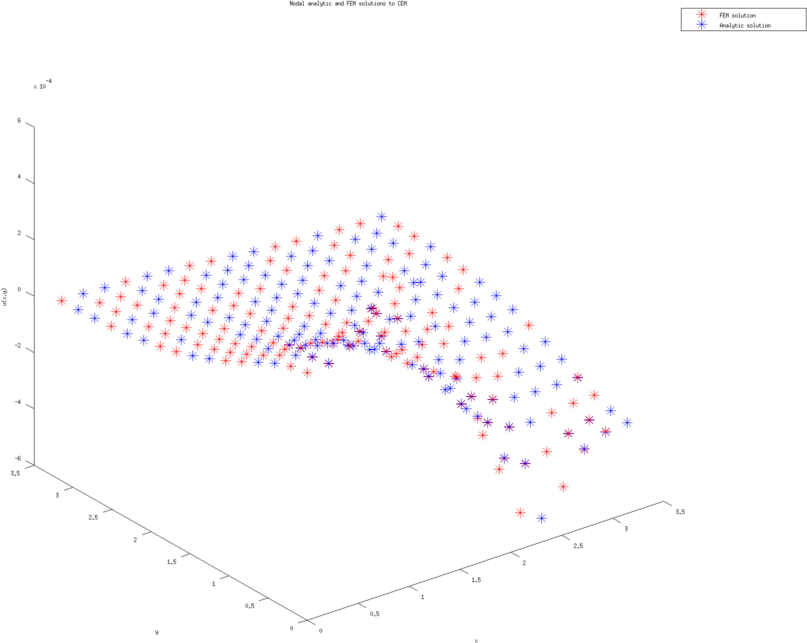
Figure: The left and right figure are the nodal potential values (with cubic approximation) using the analytic solution and finite element solution (on the coarsest triangulation.)

%Error rate fitting. 
%Assume e = Ch^{p} => log(e) = A + p log(h) and h= C(1/2)^j 
%log(e) = A+log(C) - j(p log(2)) 
%log(err) against jlog(2) will give gradient -p
n_plot=2; %First error 'not asymptotic'so disregard.

%Calculate the best fits for each z_c
for z_cj=1:length(z_c)

for j=1:nmesh
   logh(j) = j*log(2); 
   logcon_func(j)=1; 
   logquad_errL2(j,z_cj) = log(quad_errL2(j,z_cj)); logquad_errH1(j,z_cj) = ...
		 log(quad_errH1(j,z_cj)); logquad_errUM(j,z_cj)=log(quad_errUM(j,z_cj)); 
   logcub_errL2(j,z_cj) = log(cub_errL2(j,z_cj)); logcub_errH1(j,z_cj) = ...
		 log(cub_errH1(j,z_cj)); logcub_errUM(j,z_cj)=log(cub_errUM(j,z_cj));
end

%Extra data point for linear
for j=1:nmesh+1
   loglin_errL2(j,z_cj) = log(lin_errL2(j,z_cj)); loglin_errH1(j,z_cj) = ...
	 		log(lin_errH1(j,z_cj)); loglin_errUM(j,z_cj)=log(lin_errUM(j,z_cj));   
end


%Linear
Alin=[logh',logcon_func']; 
best_linL2(z_cj,:) = (Alin(n_plot:nmesh,:)'*Alin(n_plot:nmesh,:))\...
	Alin(n_plot:nmesh,:)'*loglin_errL2(n_plot:nmesh,z_cj);
best_linH1(z_cj,:) = (Alin(n_plot:nmesh,:)'*Alin(n_plot:nmesh,:))\...
	Alin(n_plot:nmesh,:)'*loglin_errH1(n_plot:nmesh,z_cj);
best_linUM(z_cj,:) = (Alin(n_plot:nmesh,:)'*Alin(n_plot:nmesh,:))\...
	Alin(n_plot:nmesh,:)'*loglin_errUM(n_plot:nmesh,z_cj);

%Quadratic
Aquad=[logh',logcon_func'];
best_quadL2(z_cj,:) = (Aquad(n_plot:nmesh,:)'*Aquad(n_plot:nmesh,:))\...
	Aquad(n_plot:nmesh,:)'*logquad_errL2(n_plot:nmesh,z_cj);
best_quadH1(z_cj,:) = (Aquad(n_plot:nmesh,:)'*Aquad(n_plot:nmesh,:))\...
	Aquad(n_plot:nmesh,:)'*logquad_errH1(n_plot:nmesh,z_cj);
best_quadUM(z_cj,:) = (Aquad(n_plot:nmesh,:)'*Aquad(n_plot:nmesh,:))\...
	Aquad(n_plot:nmesh,:)'*logquad_errUM(n_plot:nmesh,z_cj);

%Cubic
Acub=[logh',logcon_func'];
best_cubL2(z_cj,:) = (Acub(n_plot:nmesh,:)'*Acub(n_plot:nmesh,:))\...
	Acub(n_plot:nmesh,:)'*logcub_errL2(n_plot:nmesh,z_cj);
best_cubH1(z_cj,:) = (Acub(n_plot:nmesh,:)'*Acub(n_plot:nmesh,:))\...
	Acub(n_plot:nmesh,:)'*logcub_errH1(n_plot:nmesh,z_cj);
best_cubUM(z_cj,:) = (Acub(n_plot:nmesh,:)'*Acub(n_plot:nmesh,:))\...
	Acub(n_plot:nmesh,:)'*logcub_errUM(n_plot:nmesh,z_cj);
end

%Plot all linear error rate on one graph against log(z)
figure; hold on;
plot(log10(z_c),-best_linL2(:,1),'ro');
plot(log10(z_c),-best_linH1(:,1),'bx');
plot(log10(z_c),-best_linUM(:,1),'md');
h =legend('L2','H1','UM','Location','NorthWest');
set(h,'FontSize',14);
xlab = xlabel('log(z)'); set(xlab,'FontSize',14);
ylab = ylabel('Rate'); set(ylab,'FontSize',14);      
print_convert error_rates_contact_impedance03a.png

%Plot all quadratic error rate on one graph against log(z)
figure; hold on;
plot(log10(z_c),-best_quadL2(:,1),'ro');
plot(log10(z_c),-best_quadH1(:,1),'bx');
plot(log10(z_c),-best_quadUM(:,1),'md');
h =legend('L2','H1','UM','Location','NorthWest');
set(h,'FontSize',14);
xlab = xlabel('log(z)'); set(xlab,'FontSize',14);
ylab = ylabel('Rate'); set(ylab,'FontSize',14);     
print_convert error_rates_contact_impedance03b.png

%Plot all cubic error rate on one graph against log(z)
figure; hold on;
plot(log10(z_c),-best_cubL2(:,1),'ro');
plot(log10(z_c),-best_cubH1(:,1),'bx');
plot(log10(z_c),-best_cubUM(:,1),'md');
h =legend('L2','H1','I','US','UM','Location','NorthWest');
set(h,'FontSize',14);
xlab = xlabel('log(z)'); set(xlab,'FontSize',14);
ylab = ylabel('Rate'); set(ylab,'FontSize',14);      
print_convert error_rates_contact_impedance03c.png


%Plot all L2 error rates against log(z) for each approx
figure; hold on;
plot(log10(z_c),-best_linL2(:,1),'ro');
plot(log10(z_c),-best_quadL2(:,1),'bx');
plot(log10(z_c),-best_cubL2(:,1),'g+');
h =legend('p=1','p=2','p=3','Location','NorthWest');
set(h,'FontSize',14);
xlab = xlabel('log(z)'); set(xlab,'FontSize',14);
ylab = ylabel('Rate'); set(ylab,'FontSize',14); 
print_convert error_rates_contact_impedance03d.png

%Plot all H1 error rates against log(z) for each approx
figure; hold on;
plot(log10(z_c),-best_linH1(:,1),'ro');
plot(log10(z_c),-best_quadH1(:,1),'bx');
plot(log10(z_c),-best_cubH1(:,1),'g+');
h =legend('p=1','p=2','p=3','Location','NorthWest');
set(h,'FontSize',14);
xlab = xlabel('log(z)'); set(xlab,'FontSize',14);
ylab = ylabel('Rate'); set(ylab,'FontSize',14);      
print_convert error_rates_contact_impedance03e.png

%Plot all UM error rates against log(z) for each approx
figure; hold on;
plot(log10(z_c),-best_linUM(:,1),'ro');
plot(log10(z_c),-best_quadUM(:,1),'bx');
plot(log10(z_c),-best_cubUM(:,1),'g+');
h =legend('p=1','p=2','p=3','Location','NorthWest');
set(h,'FontSize',14);
xlab = xlabel('log(z)'); set(xlab,'FontSize',14);
ylab = ylabel('Rate'); set(ylab,'FontSize',14);      
print_convert error_rates_contact_impedance03f.png

> > >
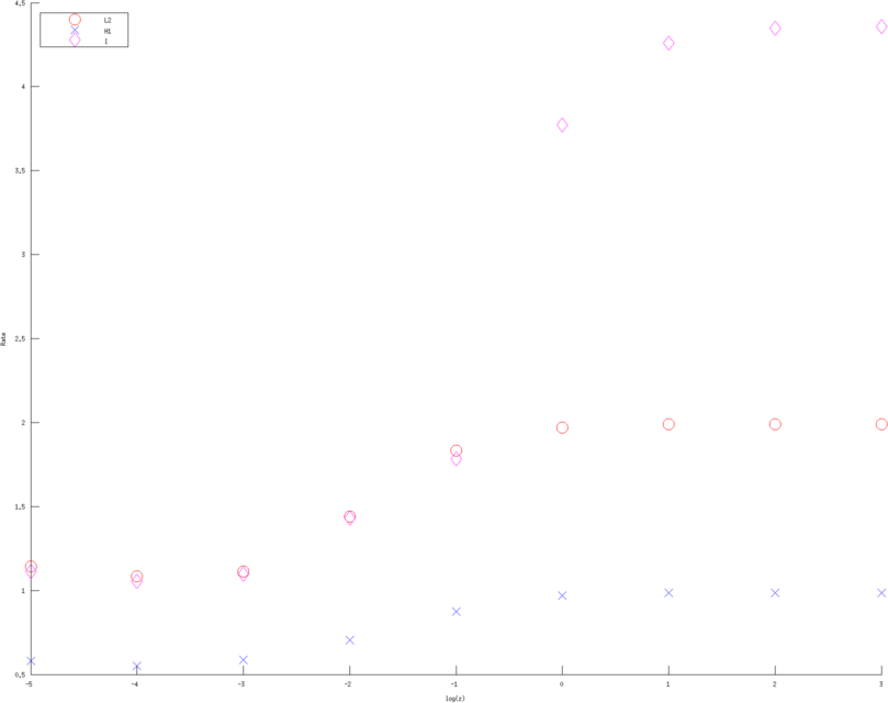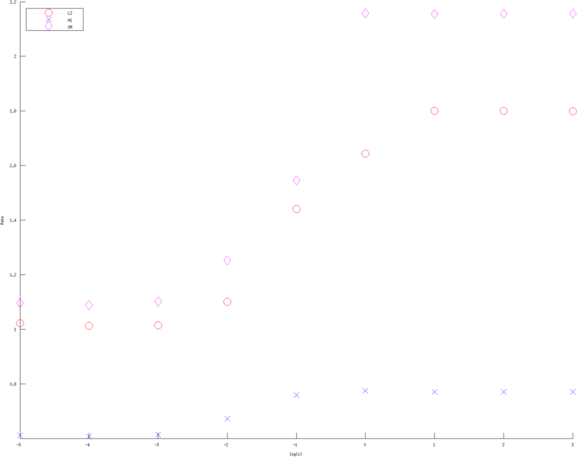
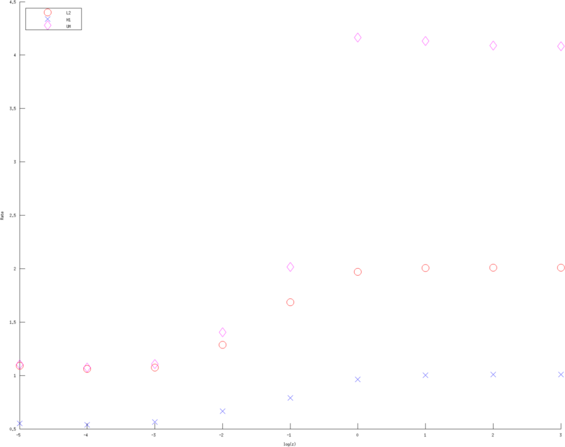
Figure: Convergence rates (of various Error norms) as a function of contact impedance for various approximation order. Left, Middle, Right figure are using a linear, quadratic and cubic approximation respectively. Bue crosses are the H1 norm, Red circle the L2 norm and Purple diamons are the measured voltages in l2 norm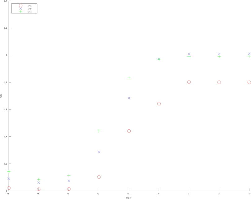

> > >
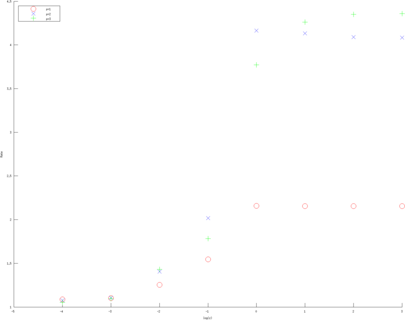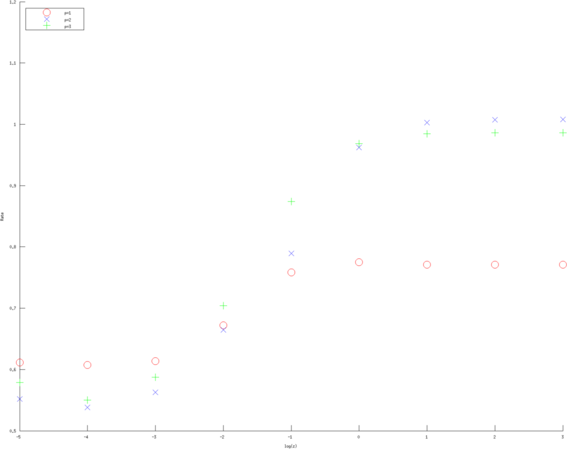
Figure: Convergence rates (of various approximation orders) as a function of contact impedance for various Error norms. Left, Middle, Right figure are error rates estimate in H1 norm, L2 norm and l2 norm of measured voltages, linear, quadratic and cubic approximation respectively. Red circles are linear, Blue diagonal crosses are quadratic and Green verticle crosses are cubic approximations.