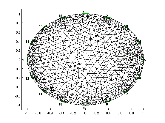
Figure: 2D model with 16 electrodes
Here are several simulated examples for the detectability of a single object. Simulations are shown below for detectability analysis in 2D and 3D (sim_2D_params.m, sim_Det_3D.m) beside GREIT parameters for a single object in 2D
function [DET, greit_para]= sim_2D_params
%%%%%%%%%%%%%%%%%%%%%%%%%%%%%%%%%%%%%%%%%%%%%%%%%%%%%%%%%%%%%%%%%%%
% sim_2D_params calculates detectability values and GREIT measures
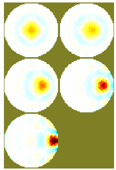
% for a single object moving from center to edge of the tank
%%%%%%%%%%%%%%%%%%%%%%%%%%%%%%%%%%%%%%%%%%%%%%%%%%%%%%%%%%%%%%%%%%%
% (C) 2011 Mamatjan Yasheng. License: GPL v2 or v3
XPos = [0:0.2:0.8]; idx=0;
for ctrx= XPos; idx=idx+1;
ctry = 0.0; brad = 0.1;
extra={'ball',sprintf(['solid ball = cylinder(', ...
'%f,%f,0;%f,%f,1;%f) and orthobrick(-1,-1,0;1,1,0.05) -maxh=0.10;'], ...
ctrx, ctry, ctrx, ctry, brad) };
[fmdl, img] = create_2D_model(extra);
ctr = interp_mesh(fmdl);
ctr=(ctr(:,1)-ctrx).^2 + (ctr(:,2)-ctry).^2;
% calculate detectability value
DET(idx) = calc_detect_val(img, brad, ctr);
% calculate simulated voltages and reconstruct images
img.elem_data = 1 + 0.01*(ctr < brad^2);
imgr(idx) = calc_volts_inv(img)
end
%
imgr(1).elem_data = [imgr(:).elem_data];
figure; show_slices(imgr(1));
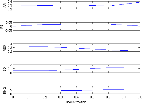
%% calculate and plot GREIT parameters
figure
YPos=zeros(1,idx); ZPos=zeros(1,idx);
xyzr_pt = [XPos;YPos;ZPos;ones(1,idx)*brad];
greit_para = calc_greit_para(imgr, xyzr_pt, XPos);
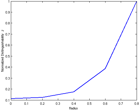
%% plot the detectability parameters
figure
plot(XPos, DET/max(DET),'linewidth',2);
ylabel('Normalized Distinguishability {\it z}');
xlabel('Radius');
end
function [fmdl, img] = create_2D_model(extra)
% create 2D model
fmdl= ng_mk_cyl_models(0,[16],[0.1,0,0.02],extra);
img= mk_image(fmdl,1);
[stim,meas_sel] = mk_stim_patterns(16,1,[0,1],[0,1],{'no_meas_current'},1);
img.fwd_model.stimulation= stim;
end
function greit_para = calc_greit_para(imgr,xyzr_pt,XPos)
% calculate and plot the GREIT PARAMETERS
greit_para = eval_GREIT_fig_merit(imgr(1), xyzr_pt);
p_names = {'AR','PE','RES','SD','RNG'};
for i=1:5; subplot(5,1,i);
plot(XPos,greit_para(i,:)); ylabel(p_names{i});
if i<5; set(gca,'XTickLabel',[]);end
end
xlabel('Radius fraction');
end
function DET = calc_detect_val(img, brad, ctr)
% calculate the detectability parameters
vol= get_elem_volume(img.fwd_model);
contr = 1e-2;
indx = zeros(size(vol));
indx(ctr < brad^2)=+ contr;
J = calc_jacobian( img );
Jr = J*indx;
DET = 1e6*sqrt( Jr'*Jr );
end
function imgr = calc_volts_inv(img)
% calculate simulated voltages and reconstruct images
imgh= img; imgh.elem_data(:) = 1;
% calculate voltages
vi = fwd_solve(img);
vh = fwd_solve(imgh);
imdl= mk_common_model('c2c2',16);
[stim,meas_sel] = mk_stim_patterns(16,1,[0,1],[0,1],{'no_meas_current'},1);
imdl.fwd_model.stimulation = stim;
imdl.fwd_model.meas_select = meas_sel;
imdl.hyperparameter.value = .001;
imgr = inv_solve(imdl,vh,vi);
end
GREIT analysis includes the figures of merit based on the GREIT algorithm (Adler et al 2009) such as (1) amplitude response (AR), (2) position error (PE), (3) resolution (RES), (4) spatial distortion (SD) and (5) ringing (RNG).
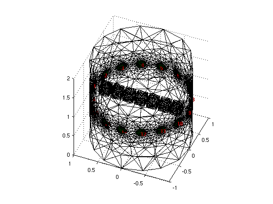
% 3D Simulatulation example of system evaluation
% (C) 2011 Mamatjan Yasheng. License: GPL v2 or v3
function [DET] = sim_Det_3D
in_plane_Def=0; % in plane or off-plane
Nelec= 16; Dims = 3; nrings = 1;
opt = {'no_meas_current'};
sp = 1; mp= 1; % stimulation, measurement
[img, vol, boxidx] = calc_fwd_cube( Dims, Nelec,in_plane_Def);
stim = mk_stim_patterns(Nelec, nrings, [0,sp], [0,mp], opt, 1);
DET = distinguishability_calc( img, stim, boxidx, vol);
plott(DET);
end
function SNR = distinguishability_calc( img, stim, boxidx, vol)
img.fwd_model.stimulation = stim;
J = calc_jacobian( img );
for ri = 1:length(boxidx);
idx = boxidx{ri};
Jr = J*idx;
SNR(ri) = 1e6*sqrt( Jr'*Jr );
end
end
function [img, vol, boxidx] = calc_fwd_cube(Dims, Nelec,in_plane_Def)
% cube moved to 7 position
if in_plane_Def %% in plane
extra={'boxes', ...
['solid box1= orthobrick(-0.1,-0.85,0.9; 0.1,-0.65,1.1) -maxh=0.05;' ...
'solid box2= orthobrick(-0.1, -0.6,0.9; 0.1, -0.4,1.1) -maxh=0.05;' ...
'solid box3= orthobrick(-0.1, -0.35,0.9; 0.1,-0.15,1.1) -maxh=0.05;' ...
'solid box4= orthobrick(-0.1,-0.1,0.9; 0.1,0.1,1.1) -maxh=0.05;' ...
'solid box5= orthobrick(-0.1, 0.15,0.9; 0.1,0.35,1.1) -maxh=0.05;' ...
'solid box6= orthobrick(-0.1, 0.4,0.9; 0.1,0.6,1.1) -maxh=0.05;' ...
'solid box7= orthobrick(-0.1, 0.65,0.9; 0.1,0.85,1.1) -maxh=0.05;' ...
'solid boxes = box1 or box2 or box3 or box4 or box5 or box6 or box7;']};
else %% off plane
extra={'boxes', ...
['solid box1= orthobrick(-0.1,-0.85,1.4; 0.1,-0.65,1.6) -maxh=0.05;' ...
'solid box2= orthobrick(-0.1, -0.6,1.4; 0.1, -0.4,1.6) -maxh=0.05;' ...
'solid box3= orthobrick(-0.1, -0.35,1.4; 0.1,-0.15,1.6) -maxh=0.05;' ...
'solid box4= orthobrick(-0.1,-0.1,1.4; 0.1,0.1,1.6) -maxh=0.05;' ...
'solid box5= orthobrick(-0.1, 0.15,1.4; 0.1,0.35,1.6) -maxh=0.05;' ...
'solid box6= orthobrick(-0.1, 0.4,1.4; 0.1,0.6,1.6) -maxh=0.05;' ...
'solid box7= orthobrick(-0.1, 0.65,1.4; 0.1,0.85,1.6) -maxh=0.05;' ...
'solid boxes = box1 or box2 or box3 or box4 or box5 or box6 or box7;']};
end
switch Dims; % dims = 2 (2D) or 3 (3d)
case 3;
fmdl= ng_mk_cyl_models(2,[Nelec,1],[0.1,0,0.03],extra);
%show_fem(fmdl, [1 1 0])
case 2;
fmdl= ng_mk_cyl_models(0,Nelec,[0.1,0,0.01],extra);
otherwise; error('huh?');
end
img= mk_image(fmdl,1);
idx = fmdl.mat_idx{2};
vol= get_elem_volume(fmdl);
ctrs = interp_mesh(fmdl); ctrs = ctrs( idx,: );
rctrs = sqrt(ctrs(:,1).^2 + ctrs(:,2).^2) ;
x= ctrs(:,1); y= ctrs(:,2); z= ctrs(:,3);
contr = 5*1e-3;
area0 = sum(vol(idx));
indx = zeros(size(vol)); list = idx(y < -0.625);
area1 = sum(vol(list));
indx(list)=+ contr*area0/area1;
boxidx{1} = indx.*vol;
% img.elem_data = boxidx{1};
% show_slices(img,1)
indx = zeros(size(vol)); list = idx( y < -0.375 & y > -0.625);
area1 = sum(vol(list));
indx(list)=+ contr*area0/area1;
boxidx{2} = indx.*vol;
indx = zeros(size(vol)); list = idx( y < -0.125 & y > -0.375);
area1 = sum(vol(list));
indx(list)=+ contr*area0/area1;
boxidx{3} = indx.*vol;
indx = zeros(size(vol)); list = idx(y > -0.125 & y < 0.125);
area1 = sum(vol(list));
indx(list)=+ contr*area0/area1;
boxidx{4} = indx.*vol;
indx = zeros(size(vol)); list = idx( y > 0.125 & y < 0.375);
area1 = sum(vol(list));
indx(list)=+ contr*area0/area1;
boxidx{5} = indx.*vol;
indx = zeros(size(vol)); list = idx( y > 0.375 & y < 0.625);
area1 = sum(vol(list));
indx(list)=+ contr*area0/area1;
boxidx{6} = indx.*vol;
indx = zeros(size(vol)); list = idx( y > 0.625);
area1 = sum(vol(list));
indx(list)=+ contr*area0/area1;
boxidx{7} = indx.*vol;
end
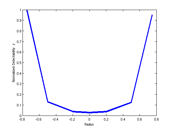
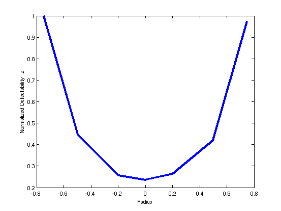
function plott(DET)
ax = [-0.75, -0.5, -0.2, 0, 0.2, 0.5, 0.75];
plot(ax, DET/max(DET),'linewidth',4)
ylabel('Normalized Detectability {\it z}');
xlabel('Radius');
end
Last Modified: $Date: 2017-02-28 13:12:08 -0500 (Tue, 28 Feb 2017) $ by $Author: aadler $